nueva página del texto (beta)
 Inglés (pdf)
 Artículo en XML
 Referencias del artículo
 Enviar artículo por email
 Citado por SciELO
  Similares en
SciELO
Similares en
SciELO 
 Permalink
1.Introduction
Ever since the discovery of first radio sources (Matthews & Sandage 1963; Schmidt 1963) in 1963, a considerable amount of work and computing resources have been invested in exploring the observable Universe to detect radio sources. Quasar and BL Lacertae objects are supermassive rotating black holes, with jet ejection and rotation axes, which emit in radio, and gamma rays. Their radio signals are observable when the axis of their emission cone is directed along the line of sight to the instrument. Subsequently, they have also been observed throughout the electromagnetic spectrum. A review of the various observational properties of quasars and other kinds of active galaxy nuclei (AGN) can be found in Véron-Cetty & Véron (2010).
AGNs, particularly quasars, have been studied at many radio frequencies to understand the mechanisms and regimes of energies involved in the phenomenon. As a result, a unified model was elaborated in which the different denominations given to the AGN are derived from the orientation of the jets in relation to the viewing angle of the observer (Antonucci 1993; Urry & Padovani 1995; Beckmann & Shrader 2012).
The variability is the aspect of AGN that attracts the most attention. Some radio sources have periodicities measured in a scale of years, but due to the delay between the measurements made in several frequencies, it is difficult to accurately specify the periodicity. Delays make it difficult to study time series when comparing light curves at different frequencies. In addition, the data set comprises a time series of irregular sampling due to various factors influencing the acquisition of astronomical data from ground stations, such as weather conditions, system maintenance, receivers, etc. These sampling difficulties produce unequally spaced time series, which impose limitations on more conventional methods of analysis.
Multifrequency studies explore distinct aspects of compact radio sources, in particular, flux density variations, to determine periodicities in light curves (Abraham et al. 1982; Botti & Abraham 1987, 1988; Botti 1990, 1994; Aller et al. 2009; Aller & Aller 2010, 2011). Methods for determining periodicities in the radio range include Fourier Transform, Lomb-Scargle Periodogram, Wavelet Transform and Cross Entropy, among others (Cincotta et al. 1995; Tornikoski et al. 1996; Santos 2007; Soldi et al. 2008; Vitoriano & Botti 2018). A combination of methods, like decision trees, random forests and autoregressive models is usual for the specific goal of exoplanets detection in stellar light curves (Caceres et at. 2019).
Advances in artificial intelligence have provided machine learning algorithms, such as neural networks, ensemble and deep learning (LeCun et al. 2015), that aid astrophysical studies and provide computational approaches dissimilar to previous methods, including potential applications for radio source analyses (Witten et al. 2016).
Motivated by the successful performance of in International Challenges on Machine Learning , and animated by the many different kinds of results presented by Pashchenko et al. (2017), Smirnov & Markov (2017), Bethapudi & Desai (2018), Abay et al. (2018), van Roestel et al. (2018), Saha et al. (2018), Lam & Kipping (2018), Shu et al. (2019), Liu et al. (2019), Askar et al. (2019), Calderon & Berlind (2019), Chong & Yang (2019), Jin et al. (2019), Menou (2019), Plavin et al. (2019), Wang et al. (2019), Yi et al. (2019), Li et al. (2020), Lin et al. (2020), Hinkel et al. (2020), Tamayo et al. (2020) and Tsizh et al. (2020), we decided to test how this kind of algorithm would perform specific tasks related to the treatment of time series in radio datasets of AGNs, such as light curves of quasars and BL Lacs. For this reason we selected two well-studied objects, the PKS 1921-293 (OV 236) quasar and PKS 2200+420 (BL Lac) for a case study.
The outline of this paper is as follows. In § 2, the AGNs datasets from the UMRAO survey, along with the features used for training and tests, are described. In § 3, we show the machine learning algorithms applied to the AGNs datasets. The implementation of XGBoost is described in detail. We discuss the feature selection procedure methods in § 4. We report and discuss the results of machine learning algorithms for the selected tasks in § 5. We present a summary and conclusions in § 6.
2.Instrument and Datasets
The Michigan Radio Astronomy Observatory (UMRAO), has a parabolic reflector antenna of about 26 meters in diameter. This radio telescope has been used extensively since 1965 to monitor continuous full-flux density and linear polarization of variable extragalactic radio source in the frequencies of 4.8 GHz (6.24 cm), 8.0 GHz (3.75 cm) and 14.5 GHz (2.07 cm). More details about UMRAO characteristics and their astrophysics applications are reviewed and can be found in Aller (1992); Aller et al. (2017).
In our study, we used UMRAO datasets for PKS 1921-293 (OV 236) and PKS 2200+420 (BL Lac), in the time intervals presented in Table 1.
TABLE 1 IRREGULARLY SPACED TIME SERIES*
| Frequency (GHz) | PKS 2200+420 | PKS 1921-293 |
|---|---|---|
| 4:8 | 1977-2012 | 1979-2011 |
| 8:0 | 1968-2012 | 1974-2011 |
| 14:5 | 1974-2012 | 1975-2011 |
*The UMRAO datasets were acquired in frequencies of 4:8 GHz, 8:0 GHz and 14:5 GHz from radio sources PKS 1921-293 (OV 236) and PKS 2200+420 (BL Lacertae).
It is worth mentioning that these are irregularly spaced time series, so the years indicated in Table 1 refer to the range of years covered in this study. The differences in the years of radio datasets start for each frequency, for both objects of study, are due to the fact that the UMRAO began to operate in each one of the frequencies in different epochs.
For all objects in the dataset collection and at all operating frequencies, UMRAO provides daily time series1. Due to several inherent aspects of observations, such as weather and instrumental maintenance, the data sets are irregularly spaced, requiring treatment before being used in the research. The procedures adopted during processing for this purpose will be described later, in § 4.
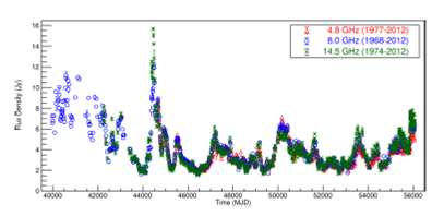
The Figures 9 and10 in Appendix A, show the light curves for the objects PKS 2200+420 (BL Lac) and PKS 1921-293 (OV 236), respectively, arranged in graphs according to the same time interval, for comparison purposes.
The characteristics of the radio source PKS 2200+420 (BL Lac)2 used in this study are galactic coordinates 92.5896 -10.4412, equatorial coordinates (J2000) RA 22h02m43,291s DE +42o16´39,98, constellation Lacerta, apparent magnitude V= 14.72, absolute magnitude MV = -22.4 and redshift z ≈ 0.069.
The characteristics of the radio source PKS 1921-293 (OV 236)3 are equatorial coordinates (J2000) RA 19h24m51.056s DE -29o14´30,11, galactic coordinates 9.3441 -19.6068, constelation Sagittarius, apparent magnitude V=17.5, absolute magnitude MV=-24.6 and redshift z ≈ 0.353 .
The UMRAO datasets are provided in digital files in the American Standard Code for Information Interchange (ASCII) coding standard and contain, listed in daily sequences, the acquisition date in modified Julian date format, the flux density and the associated measurement error, both in jansky. Table 2 shows the number of observations per frequency for each radio source addressed in this study.
3.XGBoost
XGBoost, an acronym for eXtreme Gradient Boosting, is a set of machine learning methods boosted tree based, packaged in a library designed and optimized for the creation of high performance algorithms (Chen & Guestrin 2016). Its popularity in the machine learning community has grown since its inception in 2016. This model was also the winner of High Energy Physics Meets Machine Learning Kaggle Challenge (Xu 2018). In astrophysics, XGBoost was recently used for the classification of pulsar signals from noise (Bethapudi & Desai 2018) and also to search for exoplanets extracted from the PHL-EC (Exoplanet Catalog hosted by the Planetary Habitability Laboratory)4 using physically motivated features with the help of supervised learning .
Gradient boosting is a technique for building models in machine learning. The idea of boosting originated in a branch of machine learning research known as computational learning theory. There are many variants on the idea of boosting (Witten et al. 2016). The central idea of boosting came out of the question of whether a “weak learner” can be modified to become better. The first realization of boosting that saw a great success in its application was Adaptive Boosting or AdaBoost and was designed specifically for classification. The weak learners in AdaBoost are decision trees with a single split, called decision stumps for their shortness (Witten et al. 2016).
AdaBoost and related algorithms were recast in a statistical framework and became known as Gradient Boosting Machines. The statistical framework cast boosting as a numerical optimization problem, where the objective is to minimize the loss function of the model by adding weak learners using a gradient descent like procedure. The Gradient Boosting algorithm involves three elements. (i) A loss function to be optimized, such as cross entropy for classification or mean squared error for regression problems. (ii) A weak learner to make decisions, integrating a decision tree. (iii) An additive model, used to add weak learners to minimize the loss function. New weak learners are added to the model in an effort to correct the residual errors of all previous trees. The result is a powerful modeling algorithm.
XGBoost works in the same way as Gradient Boosting, but with the addition of an Adaboost-like feature of assigning weights to each sample. In addition to supporting all key variations of the technique, the real interest is the speed provided by the implementation, including: (i) parallelization of tree construction using all computer CPU cores during training; (ii) distributed computing for training very large models using a cluster of computers; (iii)out-of-core computing for very large datasets that do not fit into memory; (iv) cache optimization of data structures and algorithms to make best use of hardware (Mitchell & Frank 2017).
The XGBoost core engine can parallelize all members of the ensemble (tree), giving substantial speed boost and reducing computational time. On the other hand, the statistical machine-learning classification method is used for supervised learning problems, where the training data with multiple features are used to forecast a target variable, and the regularization techniques are used to control over-fitting. The method uses a non-metric classifier, and is a fairly recent addition to the suite of machine learning algorithms (Chen & Guestrin 2016). Non-metric classifiers are applied in scenarios where there are no definitive notions of similarity between feature vectors.
Traditionally, gradient boosting implementations are slow because of the sequential nature in which each tree must be constructed and added to the model. XGBoost solves the slowness problem putting trees to work together, and creating the concept of forest. This approach improves the performance in the development of XGBoost and has resulted in one of the best modeling algorithms that can now harness the full capability of very large hardware platforms (cf. benchmark tests in (Zhang et al. 2018; Huang, Yu-Pei, Yen, Meng-Feng 2019)).
In a typical machine-learning problem, the processed input data try to combine a large number of regression trees with a small learning rate to produce a model as output. In this case, learning means recognizing complex patterns and making intelligent decisions based on input dataset features provided by the human supervisor.
The algorithm comes up with its own prediction rule, based on which a previously unobserved sample will be classified as of a certain type, e. g. high and low activity period, to give a pertinent example, with a reasonable accuracy. In order to appropriately apply a method (including preprocessing and classification), a thorough study of the nature of the data should be done; this includes understanding the number of samples in each class, the separability of the data, etc. Depending on the nature of the data, appropriate preprocessing and post processing methods should be determined along with the right kind of classifier for the task (e.g. binary classification or multiclass classification, LeCun et al. 2015).
XGBoost has only two distinct machine learning capabilities: regression and classification trees. All tasks and problems to be solved need be reduced to these two categories. Regression trees are used for continuous dependent variables. Classification trees for categorical dependent variables. In regression trees, the value obtained by the terminal nodes in the training data is the mean response of the observation falling in that region. In classification trees, the value obtained by the terminal node in the training data is the mode of observations falling in that region. In this research, the developed method uses both of capabilities, as will be shown in § 4.
XGBoost is readily available as a Python API (Application Program Interface), which is used in this work.5
To the best of our knowledge, XGBoost algorithms have never been used before in AGN research for regularization of time series or during the post-processing of outbursts selection candidates.
4.Method
We prepare the machine to learn the features associated with the training and test data to fill irregularly spaced time series and to identify the occurrence of outbursts in radio sources datasets from UMRAO through the machine classification algorithm XGBoost. The goal, as stated earlier, is to test the ability of the algorithm to be used in astrophysics studies of AGN-like radio sources with a reasonably high accuracy, thereby establishing the utility of this method where different approaches are useless. The classification of outbursts was done with classification tree, whilst the regularization of time series was done with regression tree.
The entire method can be summarized in the following steps: (i) obtaining and preparing the data (preprocessing); (ii) regularizing the time series; (iii) detection of outbursts; and, (iv) calculation of periodicity within defined limits of accuracy. Here we will highlight the regularization of time series and the detection of outbursts, mainly.
4.1.Preprocessing
Preprocessing is an essential preliminary step in any machine learning technique, as the quality and effectiveness of the following steps depend on it . This covers from obtaining the original UMRAO files, in ASCII digital format, to preparing the data with the application of algorithms whose purpose is to check data consistency, eliminate incomplete lines or other inconsistencies typical of experimental datasets stored in formatted files such as spurious characters, formatting, etc. All the procedures applied in this phase act directly and only on the original data, but without altering them in their fundamental characteristics. The procedure also has the purpose of removing the beginning or end of the data in the case of a big time lag to the next data, reducing the error propagation and the computational time.
The original data files of the UMRAO contain all three frequencies acquired, 4.8GHz, 8.0GHz and 14.5GHz unsorted in the file lines. Each line corresponds to a daily measurement in a given frequency. During preprocessing, rows of the same frequency were collected and stored together in a separate file. In this way, each frequency can be treated independently for each object studied.
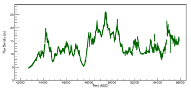
At the end of this step, the graphs of the original daily flux density data were plotted. For simplicity, only the 8.0mGHz data are shown in Figure 1 for the PKS 2200+420 (BL Lac) radio source. All other frequencies, 4.8GHz and 14.5GHz are shown in Figures 11 and12, Appendix B.

Fig. 1. Light curve of PKS 2200+420 radio source, at 8.0GHz. The raw dataset is shown. The color figure can be viewed online.
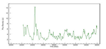
Likewise, the same preprocessing step give the result shown in Figure 2 for the PKS 1921-293 (OV 236) radio source. In this way, it was possible to visualize the segments of light curves that had most discontinuities. As before, Figures 13 and 14 for frequencies 4.8GHz and 14.5GHz are shown in Appendix B.
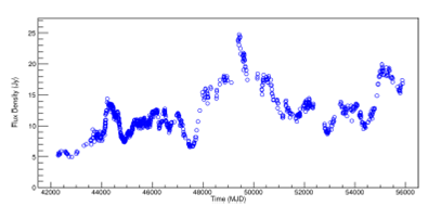
Fig. 2 Light curve of PKS 1921-293 radio source at 8.0GHz The raw dataset is shown. The color figure can be viewed online.
Notice that the time intervals for each radio source shown in Table 1 and in Figures 9 in Appendix A, differ from those shown in Figure 1 and Figures 11 and12. Also, the curves in Figure 10 in Appendix A, differ from those show in Figure 2 and Figures 13 and14. Such discrepancy is due to the head and tail elimination of the dataset effected during the preprocessing procedure.
4.2.Regularizing Time Series
The UMRAO datasets containing the individual frequencies have several time gaps configuring an irregularly spaced time series. In this method step, XGBoost was used to fill the intervals by applying machine learning regression techniques, rather than conventional techniques or methods of usual statistic adjusting. The strategy employed with XGBoost is shown in Figure 3.

Fig 3 Schematic representation of how the algorithm using XGBoost finds a missing point to fill and complete the irregularly spaced time series. The error bars can limit the search space.
In Figure 3, the black point represents the best point found, i.e., flux density value, to fill the series at that missing point. Gradually darker gray points represent the successive efforts does by the new weak learners added to the model to correct the residual errors of all previous trees to choose the point to be tested in the scenario. In this schematic representation, the darker the point, the greater its assigned weight to minimize the loss function.
The term “regression” here refers to the logistic regression or soft-max for the classification task. uses a set of decision trees as described the working principle detailed in § 3.
In the interval defined by each error value,
the algorithm search for the best value that can be set at the missing point
The method of classification was to select known points, hide them from the algorithm as the training set and use the remaining samples in the dataset as the test set (subject to artificial balancing by under-sampling the known flux density values). The points chosen by the algorithm fully match the previously hidden points for the same position in the time series. By this process, applied for all UMRAO radio sources datasets, the irregularly spaced time series, becomes a regularly spaced one.
Figure 4 shows the time series regularized for PKS 2200+420 (BL Lac) at 8.0GHz frequency, by the process described. Appendix C contains Figures 15 and16 for the frequencies 4.8GHz and 14.5GHz.
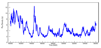
Fig. 4. Light curve of PKS 2200+420 (BL Lac) at 8.0GHz. The regularized space-time series is shown. The color figure can be viewed online.
Likewise, Figure 5 shows the regularized time series for the PKS 1921-293 (OV 236) radio source. The frequencies 4.8GHz and 14.5GHz are shown in Figures 17 and18 in Appendix C.
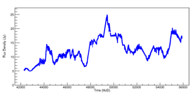
Fig. 5. Light curve of PKS 1921-293 (OV 236) at 8.0GHz. The regularized space-time series is shown. The color figure can be viewed online.
The accuracy of the regularization of the time series procedure was tested in three steps as follows. In the first step, approximately one quarter of points, constituted of flux density versus time from the original raw dataset of each frequency, are randomly chosen and put separately in different datasets for the next step. The files that contain one quarter of the points randomly extracted from the raw dataset are reserved for future comparisons. Three quarters of the raw data are put in another file to be processed by the algorithm of regularization of time series, generating another file with the regularized time series.
The file with one quarter of the randomly selected points in the first step and the file with the regularized time series generated in the second step are compared. The agreement between the separate and the new points produced by the regularization algorithm is checked through the Kolmogorov-Smirnov test (K-S Test) (Marsaglia et al. 2003; Bakoyannis 2020; Sadhanala et al. 2019; del Barrio et al. 2020).
After dataset regularization by the strategy implemented using XGBoost, any well-established statistical autoregressive model could be conveniently applied to the time series. However, we wanted to experiment and extend the use of XGBoost as much as possible and to investigate the possibilities of using machine learning also as a tool for time series regularization.
4.3.Finding Outbursts in Light Curves
In this method, XGBoost was used to classify light curve segments as probably representative of an outburst. Therefore, it is a binary classification. First, a data segment of the light curve containing a known outburst was used during the training session. Second, in the test session, the light curve of each frequency dataset was modified by the synthetic minority over-sampling technique, SMOTE (Chawla et al. 2002; Bethapudi & Desai 2018; Hosenie et al. 2020), producing a new artificial dataset, basically by introduction of noise.
By generating a known amount of the simulated noise signal and hiding it among a dataset as if being background noise, one can test if the analysis works, showing that the physics signal of the radio source is indeed detectable among the many unknown effects. It is is possible also to take note of how many false positives and negatives are introduced in each filtering step and to use those data to (a) optimize the XGBoost features and (b) evaluate the systematic uncertainly of the analysis.
The XGBoost algorithm detected peaks in the light curves at all frequencies during the training and testing processes, using the series artificially created by SMOTE. This procedure assigns a high degree of confidence to the algorithm, since it was able to identify the same peaks in the artificial and in the original light curve.
The method steps can be described as follows:
In the training and testing processes, the light curve of each frequency is already regularized by the previous step (§ 4.2). The peak of largest value was taken, assuming that it characterizes an outburst.
Preparation steps follow, including selecting samples samples covering a range of flux density with several time intervals, in days, before and after the occurrence of the largest peak in each light curve.
In the testing process, the algorithm is applied for outburst detection on the synthetic datasets created with SMOTE.
Finally, the algorithm is applied on real data sets, looking for segments of the light curve at each frequency containing, or not, an outburst; this is a binary classification.
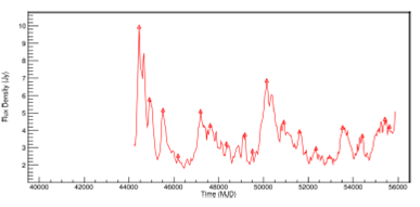
At the end of this step, the outburst candidates detected by the algorithm for PKS 2200+420 (BL Lac) at 8.0GHz were plotted as a graph, shown in Figure 6. All other frequencies for this object are shown in Figures 19 and20, Appendix D. Also shown are graphs for PKS 1921-293 (OV 236) in Figure 7 and Figures 21 and 22, Appendix D.
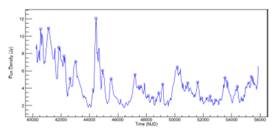
Fig. 6. Light curve of PKS 2200+420 (BL Lac) at 8.0GHz, showing the detected outbursts to periodicities found. The color figure can be viewed online.

4.4.Periodicity
The calculation to determine the periodicity takes the combination of the differences of time among all the outburst candidates identified in the classification by the XGBoost algorithm in the previous step (§ 4.3). The goal was to determine all possible combinations between the occurrences of outbursts by collecting the corresponding time intervals.
Each outburst candidate corresponds to an ordered pair of flux density with an occurrence date. The difference between all possible occurrence date combinations of all outburst candidates provides a set of time intervals, which may contain the periodicity of the phenomenon within the appropriate boundary conditions. This boundary conditions were proposed by Rasheed et al. (2011).
At this point, it is necessary to define what we considered ‘periodicity’ within the scope of this research.
Rasheed et al. (2011) distinguish between seven different definitions of periodicity. The one that interests in our context is the Periodicity with Time Tolerance. This postulates that, given a time series T which is not necessarily noise-free, a pattern X is periodic in an interval
Because it is not always possible to achieve perfect periodicity we need to specify the confidence in the reported result. Rasheed et al. (2011) define the periodicity confidence, as follows.
The confidence of a periodic pattern X occurring in time series T is the ratio of its actual periodicity to its expected perfect periodicity.
Formally, the confidence of pattern X with periodicity p starting at position startPos is defined as:
where the perfect periodicity is,
and the actual periodicity PActual is calculated by counting the number of occurrences of X in T, starting at startPos and repeatedly jumping by p positions.
Thus, for example, in
The correspondence between the time series, T, and the chain of binary digits, in which the ’1’s mark the position of the periodic pattern X occurrence in the series, helps to clarify the definition.
abbcaabcdba ccdbabbca
10000100000000010000
Applying the confidence definition (equation 3) in Periodicity with Time Tolerance like T = abce dabc cabc aabc babc c, the frequency is
The concepts as defined here were used to compute and validate the periodicities found in the datasets, T, of the radio sources examined.
The outbursts represent the periodic pattern, X. The time tolerance, tt, assumed was that of the arithmetic mean difference in days between the arrival times, to the observer, of the main outbursts at each frequency (equation 5).
This way of stipulating the time tolerance tt is based on the ansatz that any real comparison or correlation between two or more radio sources frequencies examined must take into account the temporal separation between the incoming of the characteristic peaks of the outbursts to the observer point of view.
This way of stipulating tt is as expressed in equation (2) to a temporal interval.
Figure 8 shows a synthesis diagram of the steps of the applied method, emphasizing how the aspects inherent to the use of the XGBoost and those referring to the data and to the phenomenon studied were contemplated in the design of the method.

Fig. 8 In (a) the typical algorithm of machine learning to which, whatever the purpose, any task ends up being reduced. In (b) Sequences of the general method employed. Each box in diagram (b) may have one or more steps as described in (a).
As in the case of the methodological option assumed in the regularization of time series in § 4.2, here, too, we have chosen to explore the limits of possibilities, without making use of traditional methods of calculating periodicity. For this reason, we have adopted the postulates proposed by Rasheed et al. (2011) to compute and validate the periodicities.
5.Results and Discussion
The initial methodological step, presented in § 4.1, eliminated flux density data temporally very far from each other only in the head and tail of the datasets. This process was necessary to reduce computational time of the next steps; otherwise, the time series regularization would be harder for the algorithm. As result, the time series was shortened by a few days in the head and tail. This did not bring perceptible losses to the accuracy of the method since the time series datasets were very extensive. At the head of the time series, the dates eliminated were in November of one year and in February of the following year. In the tail of the time series, the days of the following year were eliminated. Eliminating these days from the heads and tails of the time series allowed us to balance the computational time/accuracy ratio.
After refining and tuning the datasets as described above, separating frequencies into distinct files to prepare the XGBoost features was the next process.
The strategy used in the next step of the method is to have the XGBoost-based algorithm consider past and future events of flux density, to weigh and predict which flux density value within the same frequency examined is most suitable to be placed at a point missing between the past and future points of the time series.
The features delivered to XGBoost for processing in this step were prepared as a “sliding window” that traverses the points that make up the light curves of each frequency one by one, and repeating the process with each increment.
Some known points (originally existing in the time series) were hidden and the algorithm was asked to compute its value without knowing it previously as described before. The results for the p values can vary slightly due to the fact that the selected random points change with each execution of the algorithm which calculates the K-S test. Even so, the p values variation does not deviate from aproximately 99% as summarized in Table 3.
TABLE 3 RESULT OF THE K-S TEST APPLIED ON TWO SAMPLES*
| PKS 2200+420 (BL Lac) | PKS 1921-293 (OV 236) | |||
| Frecuency(GHz) | statistic | p value | statistic | p value |
| 4.8 | 0:03571429 | 0:99989572 | 0:03246753 | 0:99999660 |
| 8.0 | 0:03349282 | 0:99974697 | 0:03097345 | 0:99988705 |
| 14.5 | 0:03361345 | 0:99913286 | 0:02734375 | 0:99997300 |
*One with the raw empirical data of flux density and another calculated, for the same point, with the algorithm of regularization based on tree boosting.
The empirical data versus values calculated by the time series regularization algorithm have a very high statistical adherence of about 0.99. Thus, the K-S Test rejects the the null hypothesis that the samples are drawn from the same distribution in the two-sample case. This means that there is no evidence to say that the set of values does not adhere, so it is understood that the calculated values come from the same probability distribution, since the correlation is high in all cases. In other words, the probability of these two samples not coming from same distribution is very low. But, statistically speaking, one cannot be 100% sure.
For this reason the method of regularization based on tree boosting is used instead of conventional techniques. This process offers more convincing results than the use of more conventional techniques such as spline, that smooth too much the curves from experimental data.
The curves shown in Figure 4 (§ 4.2) and Figures 15 and16 (Appendix C) of PKS 2200+420 (BL Lac) and Figure 5 and Figures 17 and18 of PKS 1921-293 (OV 236), are actually plots of daily points, merging previously obtained points from UMRAO and points forecast by the XGBoost algorithm. This is not a line in fact. The tessellated aspect results from the fact that some values of the flux density (real or forecast) are much higher or lower than their predecessors or successors.
Table 4 summarizes the hyper parameters values with which XGBoost was configured in this step of the method.
TABLE 4 HYPER PARAMETERS OF XGBOOST MODELS*
| Number of estimators | 1000 |
| Learning rate | 0.001 |
| Maximum depth | 4 |
| Regularization alpha | 0.01 |
| Gamma | 0.1 |
| Sub sample | 0.8 |
*Used for the method applied for time series regularization discussed here.
XGBoost Python API6 provides a method to assess the incremental performance by the number of trees. It uses arguments to train, test and to measure errors on these evaluation sets. This allows us to adjust the model performance until best results in terms computational time/accuracy ratio are reached.
In Table 4, as in Table 5, the XGBoost hyper parameters are (Aarshay 2016):
Number of estimators: sets the number of trees in the model to be generated.
Learning rate: affects the computation time performance which decreases incrementally the learning rate, while increasing the number of trees.
Maximum depth: represents the depth of each tree, which is the maximum number of different features used in each tree.
Regularization alpha: is the linear booster term on weight; it controls the complexity of the model which prevents overfitting,
Gamma: specifies the minimum loss reduction required to make a node splitting in the tree. This occurs only when the resulting split gives a positive reduction in the loss function.
Sub sample: is the percentage of rows obtained to build each tree. Decreasing it, reduces performance.
TABLE 5 HYPER PARAMETERS OF XGBOOST MODELS*
| Number of estimators | 200 |
| Learning rate | 0.001 |
| Maximum depth | 10 |
| Regularization alpha | 0.0001 |
| Gamma | 0.1 |
| Sub sample | 0.6 |
*Used for the method for outburst detection. We used the same set of hyper parameters for both the non-SMOTE and SMOTE datasets.
Good performance of XGBoost-based algorithms depends on the ability to adjust the hyper parameters of the model. It took time of processing in the training and testing processes, after preparing the models features, to achieve the results shown in Figure 4 and Figures 15 and16 for the PKS 2200+420 (BL Lac) datasets, Figure 5 and Figures 17 and18 for the PKS 1921-293 (OV 236) datasets.
The XGBoost-based algorithms exhibited a potential ability for detection of outbursts in the light curves of radio sources. Even when the datasets were disturbed with artificial noise introduced by SMOTE, the XGBoost algorithm retained the ability to identify outbursts, matching previous findings in all frequencies, without noise. The robustness of the method and the solid boosted tree implementation behind the algorithms are validated by the proximity of the scores computed for different datasets of both radio sources.
Figure 6 and Figures 9 and 20 of PKS 2200+420 (BL Lac) and Figure 7 and Figures 21 and 22 of PKS 1921-293 (OV 236), show the peaks identified by the XGBoost-based algorithm, according to the methodological strategy described in § 4.4.
Table 5 summarizes the hyper parameter values with which XGBoost was configured. The hyper parameters were the same in both SMOTE simulated and non-simulated, with acquired UMRAO data. This strategy was inspired by Bethapudi & Desai (2018).
As in the previous methodological step, at this stage also it was essential to adjust the hyper parameters to obtain the results discussed here.
The use of previously adjusted datasets contributed to gain precision in the accuracity of detection of the outbursts, since it enlarged the sample space and the temporal resolution.
XGBoost, as well as other implementations of tree optimization algorithms, is a good choice for both classification and prediction. But decision tree ensemble models are not directly applicable for variability or periodicity studies. A smart strategy was required to be able to extract periodicity from the light curves using tree boosting.
In fact, the XGBoost contribution to the periodicity calculation ended with the identification of outburst candidates from the light curves. Thereafter, the method is reduced to calculate differences, subtracting all pairs of peaks found from each other, and verifying if the values found fall within a time tolerance.
The algorithm based on XGBoost was subjected to two tests. In the first, artificial datasets SMOTE were used to verify if the algorithm would find the candidate peaks of outburst, despite the introduced random combination of artificial noises by the SMOTE technique. In the second, the light curves were inverted in such a way that the first point of the curve became the last and vice versa. After re-training the algorithm, all points were identified in both cases.
Finally after the training and test procedures, the algorithm was applied to the UMRAO datasets of both object, obtaining good results.
The results were compared with those of previous works obtained using the same datasets, but with different statistical methods. In addition to the difference in method and size of the time series (which were smaller than the time series used in this work, since they were from years ago, when the datasets used here were not available) a characteristic of the works consulted is that they employed conventional ways to treat irregular time series.
The results for PKS 2200+420, shown in Table 6, are compared with the results found in several works, collected in Table 7 for the methods: Discrete Fourier Transform, Discrete AutoCorrelation Function (DFT/ACF) , Simultaneous Threshold Interaction Modeling Algorithm (STIMA) , Power Spectral Analysis Method (PSA) Villata et al. (2004), Simultaneous Threshold Interaction Modeling Algorithm (STIMA) Ciaramella et al. (2004), Power Spectral Analysis Method (PSA) Yuan (2011), Date-Compensated Discrete Fourier Transform (DCDFT) Fan et al. (2007) and Continuous Wavelet Transform, Cross-Wavelet Transform (WT) Kelly et al. (2003).
TABLE6 PERIODICITY OBTAINED FOR PKS 2200+420 (BL LAC)*
| Frequency (GHz) | Time interval | Periodicity (year) |
|---|---|---|
| 4.8 | 1978-2011 | 1:7, 3:4, 5:7 |
| 8.0 | 1969-2011 | 1:7, 3:8, 5:2 |
| 14.5 | 1975-2011 | 1:7, 2:9, 4:7 |
*After computational procedure to classify ux density segments as potential outbursts. Values with a precision of 88:95%.
TABLE 7 COMPARISON OF THE PERIODICITY OBTAINED FOR PKS 2200+420 WITH PERIODICITIES ESTIMATED BY DIFFERENT METHODS
| Time interval | Method | 4.8GHz | 8.0GHz | 14.5GHz |
|---|---|---|---|---|
| 1968-2003 | DFT/ACF | 1:4 yr | 3:7 yr | 7:5; 1:6; 0:7 yr |
| 1977-2003 | STIMA | 7:8 yr | 6:3 yr | 7:8 yr |
| 1968-1999 | PSA | 5:4; 9:6; 2:1 yr | 4:9; 9:6; 2:8 yr | 2:4; 4:3:14:1 yr |
| 1977-2005 | DCDFT | 3:9; 7:8 yr | 3:8; 6:8 yr | 3:9; 7:8 yr |
| 1984-2003 | WT | 1:4 yr | 3:7 yr | 3:5; 1:6; 0:7 yr |
The results for PKS 1921-293, shown in Table 8, are compared with the results found in the work, collected in Table 9, unlike the various works collected to compare with the result of PKS 2200+420 (BL Lac). Gastaldi (2016) made a full review in his PhD thesis about other methods to find periodicities to compare with his own method to calculate periodicities in PKS 1921-293.
TABLE 8 PERIODICITY OBTAINED FOR PKS 1921-293 (OV 236)*
| Frequency (GHz) | Time interval | Periodicity (year) |
|---|---|---|
| 4.8 | 1980-2011 | 1:2, 3:6, 5:0 |
| 8.0 | 1975-2011 | 1:3, 2:8, 5:2 |
| 14.5 | 1976-2011 | 1:6, 3:2, 6:3 |
*After computational procedure to classify flux density segments as potential outburst. Values with a precision of 89:83%.
Table 9.Periodicity obtained for PKS 1921-293 (OV 236) and periodicities estimated by the Lomb periodogram and Wavelet methods
| Frequency GHz | Time interval | Method | Periodicity (year) |
|---|---|---|---|
| 4.8 | 1980-2006 | Lomb | 1:8, 3:3, 9:5 |
| Wavelet | 1:2-1:9, 2:7-2:8, | ||
| 5:2-5:3 | |||
| 8.0 | 1981-2006 | Lomb | 1:3, 2:8, 3:0, 5:0, |
| 8:5u | |||
| Wavelet | 1:2-1:4, 2:3-2:6, 3:2, | ||
| 4:3-5:1 | |||
| 14.5 | 1982-2006 | Lomb | 1:3, 2:5, 4:3, 6:5 |
| Wavelet | 1:3-2:3, 3:6, 5:0-5:5 |
When comparing the results of Table 6 with Table 7 and of Table 8 with Table 9, it is noted that they are similar. It is recommended to keep in mind that the time series intervals are different and smaller than those used in this paper. In spite of this, and of the methods used in the manner in which the data are processed, it is seen that the periods are similar, in particular those of the frequency 14.5GHz of the PKS 2200+420 radio source.
These results can only be considered compatible if a time tolerance limit is assumed, estimated through the arrival delay of the maximum peaks of the several frequencies at the observer. The value of this delay for PKS 1921-293, is, on average, approximately 42 days, and circa 21 days for PKS 2200+420.
6.Summary and Conclusions
In order to implement, test and improve a method that incorporates the tree boosting-based machine learning algorithm (XGBoost) for the analysis and study of characteristics of radio sources, and to figure out the potential capabilities that this specific tool has for astrophysics purposes, two typical datasets of radio sources are explored in the form of time series. The objects chosen were PKS 1921-293 (OV 236) and PKS 2200+420 (BL-Lac), because they were the most studied in the radio range and for which several attempts to discover the periodicity were performed by different methods. The datasets from University of Michigan Radio Astronomy Observatory (UMRAQ), which operates at frequencies of 4.8GHz, 8.0GHz and 14.5GHz were chosen.
A boost-based algorithm was tested. The method consists of using XGBoost in two different steps. In the first this machine learning library was exploited in its potential to act as a regression tool and thus to regularize non-spaced temporal series, making them regular. In the second, the potential of XGBoost as a classification tool was emphasized to select regions in the light curves that mark outbursts. In both cases the researcher expertise is an indispensable component of the success of the methodological process.
XGBoost shows precise probabilistic results, as long as the researcher has a good understanding of the problem and clearly specifies the characteristics of the phenomenon to be studied through well-defined boundary conditions and a validity and tolerance interval of well-established values in the features.
The success or failure of using XGBoost-based algorithms depends on the researcher’s skills to adjust the hyperparameters of the model. It should be noted that XGBoost cannot be used by itself for periodicity detection or calculation, such as some statistical methods or other Fourier derivative methods. The method uses the strategy of classifying outbursts in the light curve, a task viable for XGBoost, and later calculating the temporal difference between the candidates to an outburst identified by XGBoost, using a confidence interval that establishes the precision and thus, in spite of discrepancies falling within the interval, finding periodic values.
The results found were quite close to those found by other, more orthodox, methods. They have the advantage of low computational time, and the potential to be applied to big datasets.
In this first approximation of XGBoost to astrophysics through the study of radio sources, the great potential of this algorithm, and of machine learning in general, was perceived. The present results, by themselves, justify investigating other potential uses for this tool.
Future perspectives involve the extension of the study for other energy ranges, such as X-rays and gamma rays, and the exploration of the use of methods based on tree boosting and other machine learning techniques that allow for application in multifrequency analysis .
It is also expected to associate the tree boosting with XGBoost with the Monte Carlo technique to evaluate how well the available models are able to describe energy regimes, variability, and other aspects of radio sources.