


 text new page (beta)
 English (pdf)
 Article in xml format
 Article references
 Send this article by e-mail
 Cited by SciELO
  Similars in
SciELO
Similars in
SciELO 
 Permalink
1. INTRODUCTION
Mars has already been the final destination and target of observation of several missions and the interest for this planet has been growing. Among the many missions planned for the red planet, some have the exploration or observation of its moons, Phobos and Deimos, as important stages of the mission. Studying these moons remains interesting today, as there are many speculations about their origin. Among some assumptions, it is possible that they may have been formed by the agglomeration of parts of an old body that collapsed, or that they were formed by the ejection of material from Mars. They could also be captured primitive bodies, such as comets or asteroids. In this case they may contain information about the formation of the Solar System (Oberst et al. 2014). The problem in planning missions to these moons is that they have masses much smaller than Mars. This feature makes the spheres of influence (Araujo et al. 2008) of both moons to be just above or even below their surfaces (Gil & Schwartz, 2010), making it very difficult to keep a spacecraft in orbit. Alternative and appropriate forms for a spacecraft to orbit these moons were studied (Wiesel 1993) without the use of auxiliary thrusters, because this technique would lead to an increase in cost with a consequent decrease in the duration of the mission. Among the possible alternatives, there are some types of natural orbits that can be found in systems with major mass differences between the bodies. These types of orbits can be found using the circular and elliptical cases of the restricted three-body problem and using the small gravitational interaction of the moon to keep the spacecraft close to it, as if it were actually orbiting the body. In any case Mars dominates the motion of the spacecraft. They are called “Quasi-Satellite Orbits” (QSO) (Benest 1976; Kogan 1989, 1990; Lidov & Vashkov’yak 1993, 1994; Mikkola et al. 2006; Gil & Schwartz 2010). Their use has been considered for future missions to the moons of Mars. Some examples of these types of missions are: Phobos and Deimos and Mars Environment (PADME) (NASA, 2018), DePhine - Deimos and Phobos Interior Explorer (Wiesel 1993) and Martian Moons Explorer (MMX) mission (Campagnola et al. 2018). There are also cases where the spacecraft can be placed at large distances from the moon and in retrograde motion, which are the so called “Distant Retrograde Orbits” (DRO) (Lam & Whiffen 2005; Villac & Aiello 2005; Whiffen 2003). Quasi-periodic orbits located further away can also be found around other bodies of the Solar System, like Mercury, as shown in Ma & Li, (2013). In the Solar System it is also possible to find different types of orbits around moons, as can be seen in Carvalho et al. (2012), Gomes & Domingos, (2016), Santos et al. (2017) and Cinelli et al. (2019). Phobos, the largest and closest moon of the Martian system, has been the main objective of many studies (Gil & Schwartz 2010). The main goal of the present paper is to show some differences and also peculiarities of orbits around Deimos, the smallest and most distant moon of Mars. The average radius of Deimos is 6.2 km (JPL/NASA, 2019a) and its distance from Mars is 23,458 km (JPL/NASA, 2019b). It is highly non-spherical and very much like Type I and II asteroids, which are composed of rocks rich in carbonaceous material. The eccentricity of the orbit of Deimos is small.
To study how to observe Deimos using QSO-type orbits, a numerical search will be performed and the orbits will be selected according to the measured values of the maximum, minimum and average distances between the spacecraft and Deimos over a certain time. In that sense, maps of those quantities will be obtained to help to find adequate orbits.
The purpose of these measurements is to offer ranges of options (not just stand-alone orbits) for a mission to Deimos. In particular, it is desired to find mid-range orbits to place a spacecraft when it arrives in the system. Those orbits are very adequate to make the first measurements of Deimos before a closer orbit is selected. An orbit that causes the spacecraft to oscillate between distances from 40 to 200 km from the center of Deimos is considered to follow this criterion. This is a study similar to the one for Phobos in Cavalca et al. (2018). The goal is to complete the study of orbits to observe both moons of Mars. It is interesting for a mission to have some variations in the distance between the spacecraft and Deimos, because in this way it is possible to observe the moon from different locations. It is also important not to go too close to the moon, to avoid a risk of collision, while going too far from the moon increases the risk that the spacecraft will escape from the vicinity of Deimos. In that sense, mid-range orbits are adequate, because they allow the spacecraft to approach Deimos at a distance as short as possible, without the risk of crashing. In particular, Deimos has a very irregular shape and these types of orbits are also interesting because they are located at a safe distance from collision, and they are not much affected by the shape of Deimos. The idea is to use these mid-range orbits to make the first scientific observations of Deimos, to measure its gravitational field with more accuracy and to better analyze its surface. After these preliminary analyses the aim is to prepare a final approach to Deimos placing the spacecraft in lower orbits, or even landing on its surface. Some related examples can be found in Zamaro & Biggs, (2016), Akim et al. (2009) and Tuchin (2008).
To describe the motion of the spacecraft around Deimos and Mars, the restricted planar elliptic threebody problem (Szebehely 1967; Domingos et al. 2008) added to the acceleration due to the nonspherical shape of Mars, represented by the term J 2 (Sanchez et al. 2009) is used. In this model, Mars is called the primary body, because it has the largest mass of the system. Deimos is called the secondary body. Finally, the spacecraft is assumed to have a negligible mass. The primary and secondary bodies, Mars and Deimos, rotate in elliptical orbits around their common center of mass. The spacecraft travels around these bodies without influencing them. In addition to the gravitational force, we will also consider the effects of the non-spherical form of Mars, by adding the J 2 term of its gravitational potential. The non-spherical shape of Deimos is not included in the model because it has only very small effects at the distances considered in the present paper. Another objective of this paper is to measure the individual contribution of each force included in the mathematical model of the final trajectories. This is done by measuring the effect of each force during the integration time. This type of study was made for the gravity field of the Earth in Sanchez, Prado & Yokoyama (2014), and adapted for the Mars-Phobos system in Cavalca et al. (2018). The present paper will study different possibilities for the mathematical model to show the relevance of certain parameters in the search for mid-range trajectories around Deimos.
The results will be shown in color maps where it is possible to identify the maximum, minimum and average distances spacecraft-Deimos as a function of the initial conditions of the spacecraft with respect to Deimos. From these results the mission designer can select the most appropriate orbits according to the goals of the mission. It is also possible to identify regions and families of orbits with certain characteristics. The influence of the position of Deimos with respect to Mars in the trajectories will also be studied. In this case, two opposing positions will be considered: periapsis and apoapsis.
The present paper has the following objectives:(i) to find and classify orbits to observe Deimos, which can keep a spacecraft in mid-range distances from Deimos over a given time; (ii) to measure the importance of the eccentricity of the orbit of Deimos, even if small, in the orbits found; (iii) to investigate the contribution of each force that acts in the dynamics of the system, and so to be able to measure which ones are the most relevant; (iv) to analyze the effects of the initial position of Deimos with respect to Mars in the trajectories of the spacecraft.
2. MATHEMATICAL MODEL
Next, the mathematical model, the parameters and other data used and calculated during the simulations are presented, as well as the forces that influence the dynamics of the system, and the criteria to select and classify the orbits. The main idea is to build general maps that can show different possibilities of orbits. Thus, these maps can serve as catalogs, to be used according to the mission requirements, contributing to the choice of the best parameters to accomplish a mission. First, the initial conditions of the spacecraft relative to Deimos are chosen, that is, the initial distance between the spacecraft and Deimos and the initial components of the velocity v x and v y of the spacecraft. Then, the trajectory is numerically integrated over the given time. Next, the distances spacecraft-Deimos during the whole period of the natural trajectory are calculated. Then the averages, minimum and maximum distances reached by the spacecraft from Deimos are shown. Each type of orbit can be used for a certain stage of a mission. The results show that the average distances follow the same behavior of the maximum distances, while the minimum distances present small variations.
Equations 1 and 2 are the equations of motion of the spacecraft according to the model adopted. The first two terms of the equations refer to the restricted elliptic three-body problem, where m 1, m 2 and m 3 are, respectively, the masses of Mars, Deimos and the spacecraft. Mars and Deimos, called M 1 and M 2, rotate in elliptical orbits around their center of mass. The spacecraft, called M 3, travels around these bodies and in the same plane, but without influencing the motion of M 1 and M 2. The third terms of the right side of the equations refer to the acceleration due to the non-spherical shape of Mars, represented by the term J 2 of its gravity field (Sanchez et al. 2009).
where the universal gravitational constant is indicated by G; r 1 is the distance from the spacecraft to M 1 (Mars); r 2 is the distance from the spacecraft to M 2 (Deimos); the radius of Mars is r M1 ; and the position of the spacecraft is indicated by x, y.
Then, the process to obtain the desired orbits starts by choosing the values of the initial conditions, position and velocity, and the total integration time of each orbit. During the integration the average, maximum and minimum distances spacecraftDeimos are calculated. This is repeated for each orbit. Finally, the distances are classified and used to build maps. Equation 3 shows the calculation of the average distance spacecraft-Deimos (r avg) (Prado 2015), where r 2 is the distance between the spacecraft and Deimos and the total integration time is given by T.
Next, the algorithm used to search for the natural orbits around Deimos is described. At first, Mars and Deimos are assumed to be fixed on the x-axis in the fixed reference system. A spacecraft is placed in this same system and aligned in the x-axis, at a given distance from Deimos. Since all orbits intersect the x-axis at some point, conducting a search restricted to this line is enough to map all the orbits around Deimos. Figure 1 shows, in the inertial system, Mars, Deimos and the spacecraft, as well as the initial conditions (position and velocity), which identify each orbit: D, the initial distance between the spacecraft and Deimos; and v x and v y, the components of the initial velocity of the spacecraft.
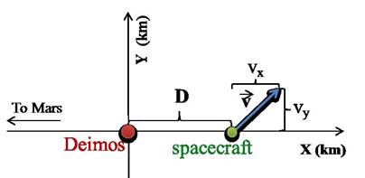
Fig. 1 Illustration of the problem showing the MarsDeimos system and the initial conditions that define each orbit: the initial distance between Deimos and the spacecraft on the x-axis is indicated by D; and the components of the initial velocity of the spacecraft are indicated by v x and v y. The color figure can be viewed online.
Based on Figure 1, it is possible to calculate the complete set of initial conditions of the spacecraft and then to make the numerical integrations of the equations of motion over the given time. During the numerical integrations the possibility of collisions of the spacecraft with Deimos is tested. The averages, minimum and maximum distances between the spacecraft and Deimos are calculated for each trajectory. These results are presented in the form of maps that will assist the mission designer in selecting the most appropriate orbits for each stage of the mission. The classification of those orbits shows orbits that are close to Deimos, but that respect some given limit to avoid collisions and escapes. On the other hand, it is possible to identify orbits that stay at longer distances from Deimos, including some that leave the neighborhood of Deimos. This type of orbit can be used to naturally transfer the spacecraft from an orbit closer to Deimos to an orbit around Mars located far from Deimos. Depending on the purpose of the mission, near or distant orbits can be selected as ideal. To have a better view of the trajectories, they will be plotted in the fixed and rotating system.
The study of the contribution of each force that acts in the system, which is made by integrating each force along the time, is presented. It follows Prado (2013), who studied the perturbation suffered by a spacecraft by the gravity fields of the Sun and the Moon. (For different systems and situations see also Prado 2014; Sanchez & Prado 2017; Sanchez, Howell & Prado 2016; Short et al. 2016; Santos et al. 2015; Oliveira et al. 2014; Oliveira & Prado 2014; Carvalho et al. 2014). Four types of integrals can be used to identify different aspects of the problem. These integrals are given by:
where a
v
=<
a
,
where
Where
Here, a indicates the acceleration due to the force under study; v the velocity of the spacecraft; A k the difference between the total acceleration and the Keplerian term of the acceleration, considering the same set of initial conditions and time; and T the final time of integration of the trajectory. The bold letters indicate vectors. The trajectory can be calculated for any desired time and the greater the time the greater the value of the integral. To exemplify, we can choose two trajectories close to Deimos, with only one of them colliding with Deimos. Analyzing only the value of the integral we could conclude that the trajectory that does not collide would be more disturbed than the other, because the integration time was smaller. In order to avoid this error, the value of the integral is multiplied by the normalization factor 1/T. Using this technique it is possible to compare trajectories with different durations.
For this work, the first type of integral is used, which consists in measuring the total acceleration suffered by the spacecraft. The second type of integral measures the variation of energy of the spacecraft due to each force. If it is negative, the force removes energy from the spacecraft. Otherwise, when it is positive, energy is added to the spacecraft. The third type of integral is calculated for each component of the acceleration. It also considers compensation for negative and positive effects. The fourth type of integral measures the difference between the accelerations of a Keplerian orbit and a disturbed orbit having the same initial conditions. Studies that use the first and second type of integral in the construction of perturbation maps, whose objective is to identify regions of low perturbations, can be found in Sanchez, Howell & Prado, (2016).
3. RESULTS
In this section, the results of the simulations are presented, considering several sets of initial conditions. Initially, a 30-day integration time is considered for the orbit, like in Gil & Schwartz, (2010) and Cavalca et al. (2018), to keep the same values used in the literature in order to compare the results. Longer times will be tested later. Table 1 shows the orbital and physical parameters of Mars and Deimos found in the JPL HORIZONS System3.
TABLE 1 PHYSICAL AND ORBITAL PARAMETERS OF MARS AND DEIMOS
| Celestial | Average | GM | J 2 | Semi-major | Eccentricity |
|---|---|---|---|---|---|
| Body | radius (km) | (km3/s2) | axis (km) | ||
| Mars | 3396.19 | 42828.0 | 0.00195 | − | − |
| Deimos | 6.2 | 9.85 × 10⁻⁵ | − | 23458 | 0.0002 |
Combining the possible values of the initial conditions of the spacecraft relative to Deimos (D and the components of the velocity v x and v y), many figures can be drawn. The figures are presented in the form of color maps, showing the minimum, maximum and average spacecraft-Deimos distances. The regions indicating collisions of the spacecraft with Deimos are shown in white. Using those maps it is possible to identify the regions of interest and, if necessary, to make a more detailed search using smaller steps for the variables to find more accurate initial conditions. Some of the trajectories are also plotted to analyze their behavior.
Initially, the simulations consider the most complete model, where Mars has a non-spherical shape and Deimos is in an eccentric orbit. Afterwards, a new simulation is performed considering the same set of initial conditions, but with Mars having a spherical shape and Deimos in a circular orbit. In this way it is possible to analyze the influence of each force on the trajectory of the spacecraft and to compare the results with a more realistic model. The study of the integrals of the accelerations present in the dynamics is also made, to quantify the contribution of each force acting in the trajectory of the spacecraft.
Figures 2 and 3 show the maximum (D max), minimum (D min) and average (D avg) distances between the spacecraft and Deimos. The distances are presented as a function of the initial distance D (km) on the horizontal axis and the velocity v x (km/s) on the vertical axis. The orbits begin at the moment when Deimos is at periapsis. The choices of these parameters are made after preliminary simulations varying all the parameters of the initial conditions and then selecting the most interesting ones. For the initial velocity v y it was observed that a fixed value of −0.003 km/s generated orbits that were at short and mid-range distances from Deimos. For the initial distance, the range D from 40 to 50 km showed to be adequate, as was a range of values for v x from −0.003 to 0.003 km/s. There were 35,760 trajectories that survive for up to 30 days and 24,340 trajectories not surviving that long, making a total of 60,100 trajectories. Each orbit is identified by a point on the graph that gives a specific value of D (horizontal axis) and v x (vertical axes). Using this technique, it is possible to show the distances spacecraft-Deimos to select the orbits of interest. The values of D max, shown in Figure 2(a), range from 80.24 to 22,330.45 km. The values of D min, Figure 2(b), go from 16.00 to 45.43 km. The values of D avg, Figure 2(c), go from 61.66 to 10,553.13 km. From the figures it is possible to identify that the trajectories that remain closer to the moon are located in the central part of the plot, where the lowest values of D max (Figure 2a), below 200 km, are located. This corresponds to 22.55% of the total number of solutions (the solutions that end in collisions divided by the number of solutions that survive for 30 days). The lowest values of D avg (Figure 2c), below 100 km, correspond to 22.33% of the total solutions. It is also observed that there is a correspondence in the dispersion of the orbits, for both the closer and the distant ones. There is also symmetry with respect to the y axis for v x equal to zero. However, the minimum distance values, Figure 2c, behave almost inversely when compared to the maximum and average values. The highest values of D min, between 40.00 and 45.46 km, are located in the same region where D max and D avg have the lowest values. These trajectories are close to Deimos, but at safe distances from it, to avoid risks of collision. These trajectories are excellent options to place a spacecraft. The lowest values of D min, which are between 16.00 and 20.00 km, can be found, in most cases, at the limits between the areas of high values of D max (over 200 km) and D min (over 100 km) and areas that indicate a collision, the blank areas. This indicates that these regions are not good options for the spacecraft: they take the spacecraft far away from the moon, but can, sometimes, pass very close and even collide with Deimos. Figures 2(d) and 2(e) show the trajectory with maximum D max. The initial conditions are: D = 49.9 km, v x = 0.0012 km/s, v y = −0.003 km/s and two simulation times were used: 30 and 150 days. They show clearly that the spacecraft goes away from Deimos and enters an orbit around Mars that is co-orbital with Deimos. Figures 3(a), 3(b) and 3(c) show results corresponding to Figures 2(a), 2(b) and 2(c), but now the model does not consider the effects of the flattening of Mars. The main difference is the reduction of the central blue region, which means that the maximum distances increase in this region. It happens for maximum and average distances. Therefore, the flattening of Mars helps to keep the orbits closer to Deimos in this region.
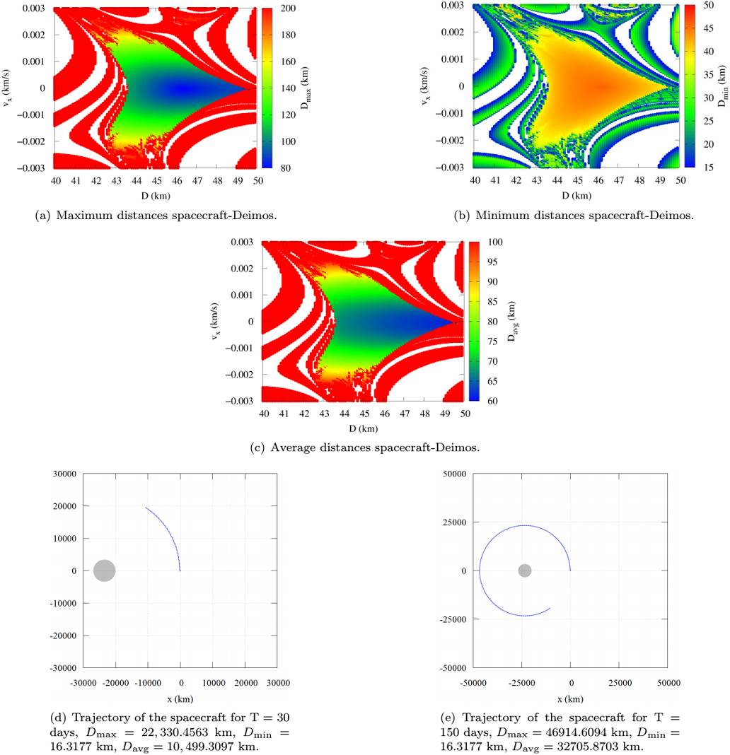
Fig. 2 Maximum, minimum and average spacecraft-Deimos distances, in km, as a function of D (km) and v x (km/s), considering vy = -0.003 km/s and that Deimos is at the periapsis of its orbit around Mars. Parts (d) and (e) show the trajectory with maximum D max. The color figure can be viewed online.
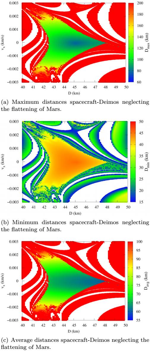
Fig. 3 Maximum, minimum and average spacecraft-Deimos distances, in km, as a function of D (km) and vx (km/s), considering vy = -0.003 km/s. The model considers e = 0, J2 = 1960.45 × 10−6, and T = 30 days. The color figure can be viewed online.
Table 2 shows the values of the maximum, minimum and average distances for the five closest orbits to Deimos, that is, those with lowest values of D max. Note that the trajectories keep the spacecraft in the distance range 80.24-80.36 km from Deimos over 30 days, without the need of orbital maneuvers. This means that they are good options to place the vehicle. The values corresponding to the model where Deimos is in a circular orbit and Mars has spherical shape are also presented, indicated by an asterisk (∗). Analyzing the differences between the values of the most complete and the simplest model, one can see the importance of considering a more realistic model. Note that, when considering spherical bodies and circular orbit for the moon, the errors are of the order of 4.33 to 4.94 km for the maximum distances; 2.44 to 2.55 km for the minimum distances and 2.33 to 2.35 km for the mean distances, over a period of 30 days. Note also that, when considering the simpler model, the values of maximum distances are overestimated. This is shown by the negative values of the last column of Table 2. The values of the mean and minimum distances are underestimated, as shown by the positive values in Columns 9 and 10 of Table 2. Figure 4 shows the trajectories with both models obtained with the data given by the first line of Table 2. The trajectories for the other lines of the table are very similar and they are omitted here. The left side considers the best model (elliptical orbit for Deimos and a flat body for Mars) and the right side the simplified model (circular orbit for Deimos and a spherical body for Mars). Note that the best model gives a near periodic orbit, while the simple model gives an orbit with some oscillations in the spacecraft-Deimos distance.
TABLE 2 THE FIVE ORBITS WITH SMALLEST D max (km) AROUND DEIMOS1
| D | vx | Davg | Dmin | Dmax | D∗avg | D∗min | D∗max | Davg − D∗avg | Dmin − D∗min | Dmax − D∗max |
|---|---|---|---|---|---|---|---|---|---|---|
| (km) | (km/s) | (km) | (km) | (km) | (km) | (km) | (km) | (km) | (km) | (km) |
| 46.4 | 0 | 64.0228 | 45.3666 | 80.2416 | 61.6881 | 42.8124 | 85.1829 | 2.3347 | 2.5542 | −4.9413 |
| 46.3 | 0 | 64.1237 | 45.4357 | 80.2701 | 61.7661 | 42.9782 | 84.6516 | 2.3576 | 2.4575 | −4.3815 |
| 46.4 | −0.00001 | 64.0212 | 45.3513 | 80.3273 | 61.6866 | 42.8118 | 85.1780 | 2.3346 | 2.5395 | −4.8507 |
| 46.4 | 0.0001 | 64.0258 | 45.3519 | 80.3292 | 61.6914 | 42.8115 | 85.1919 | 2.3344 | 2.5404 | −4.8627 |
| 46.3 | 0.00001 | 64.1268 | 45.4206 | 80.3681 | 61.7693 | 42.9774 | 84.7016 | 2.3575 | 2.4432 | −4.3335 |
1Assuming vY = -0.003 km/s, Deimos initially at periapsis, e = 0.0002, J2 = 1960.45×10−6, T = 30 days. Corresponding results for the circular and spherical model are represented by an asterisk (∗).
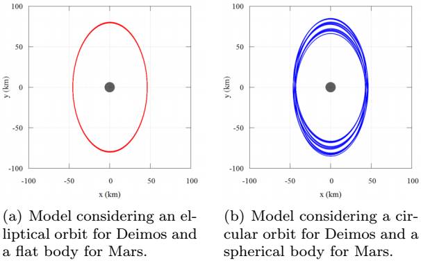
Fig. 4 Trajectories associated with the first line of Table 2 in the rotating frame. The color figure can be viewed online.
Table 3 shows the comparison between the simplified and the more complete model, over 30 days. In this case, the simplified model is used as a reference. Note that the trajectories with the lowest values of maximum distances have initial conditions different from those of Table 2, where the reference case used the most complete model. The lowest maximum distance for the complete model shown in Table 2 occurs for D = 46.40 km and v x = 0 km/s, and the value is D max = 80.24 km. The lowest maximum distance obtained when considering the model simulated in Table 3 occurs for D = 45.10 km and v x = 0.00 km/s, and it is D max = 78.40 km. Considering this last set of initial conditions for the most complete model, we have a maximum distance of 91.73 km. In Table 3, the five closest trajectories are presented considering v y = −0.003 km/s, a circular orbit for Deimos and a spherical shape for the bodies. The simulation time is equal to 30 days. The corresponding results considering the most complete model are indicated by D # max. The values of D max−D # max vary from −12.18 to −13.33 km, that is, they are all negative, which shows that the values of D max are underestimated for the orbits near Deimos. This important fact should be noted.
TABLE 3 THE FIVE ORBITS WITH SMALLEST D max (km) AROUND DEIMOS*
| D | vx | Davg | Dmin | DMAX | D*avg | D*min | D*max | Davg − D*avg | Dmin − D*min | Dmax − D*max |
|---|---|---|---|---|---|---|---|---|---|---|
| (km) | (km/s) | (km) | (km) | (km) | (km) | (km) | (km) | (km) | (km) | (km) |
| 45.1 | 0 | 62.8565 | 45.0877 | 78.4059 | 65.5536 | 44.2349 | 91.7359 | −2.6971 | 0.8528 | −13.3300 |
| 45.2 | 0 | 62.7707 | 45.0094 | 78.4426 | 65.4260 | 44.3376 | 90.6978 | −2.6553 | 0.6719 | −12.2552 |
| 45.1 | 0.00001 | 62.8581 | 45.0678 | 78.5177 | 65.5567 | 44.2349 | 91.6955 | −2.6986 | 0.8329 | −13.1778 |
| 45.1 | −0.00001 | 62.8565 | 45.0678 | 78.5178 | 65.5519 | 44.2349 | 91.7801 | −2.6954 | 0.8329 | −13.2623 |
| 45.2 | 0.00001 | 62.7722 | 44.9944 | 78.5269 | 65.4291 | 44.3370 | 90.7108 | −2.6569 | 0.6574 | −12.1838 |
*Assuming vY = −0.003 km/s, circular orbit for Deimos and spherical shapes for the bodies and T = 30 days. Corresponding results for the elliptical and flat body models are represented by D# MAX . Deimos is assumed to be initially at periapsis.
Next, Figure 5 shows the trajectories with both models, obtained with the data of the first line of Table 3. The trajectories for the other lines of the table are very similar and they are omitted here. The left side considers the best model (elliptical orbit for Deimos and a flat body for Mars) and the right side the simplified model (circular orbit for Deimos and a spherical body for Mars). Note that the simple model gives a near periodic orbit, while the best model gives an orbit with some oscillations in the spacecraft-Deimos distance.
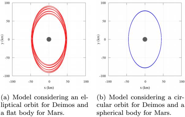
Fig. 5 Trajectories associated with the first line of Table 3 in the rotating frame. The color figure can be viewed online.
To show the influence of each force on the dynamics of the system, the integral tests will be carried out (Prado 2013). These tests are performed integrating the individual acceleration of each force for the total time of the trajectory, and then dividing it by the total integration time. In Sanchez, Prado & Yokoyama, (2014) a similar study was made for another system. Dividing the total result by the integration time, we obtain the average effect of each force acting during the whole trajectory. Using this information it is possible to identify the importance of each force.
Figure 6 shows the contribution due to Deimos, in km/s2, using the same initial conditions of Figure 2. The effect due to the gravity of Deimos (PertDeimos) varies from
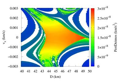
Fig.6
Perturbation due to Deimos in
The next step is to verify the behavior of those orbits over longer times. Table 4 shows the distance (km) and the disturbance level (km/s2) for simulation times of 5, 15, 30, 60, and 90 days. It is clear that some QSOs can “survive” for longer periods of time. The model considered has an elliptical orbit for Deimos and a flat Mars, so e = 0.0002 and J 2 = 1960.45 × 10−6, and Deimos at periapsis when the motion starts. The initial conditions of the trajectory are: D = 46.4 km, v x = 0 and v y = −0.003 km/s. The values of distances and perturbations remained stable during the time simulated. Remember that each individual result of the integrals of the accelerations is divided by the total integration time, to obtain a normalized number.
TABLE 4 TEMPORAL EVOLUTION OF A SINGLE ORBIT WHIT DEIMOS AT PERIAPSIS*
| T (days) | 5 | 15 | 30 | 60 | 90 |
| DMAX (km) | 80.2362 | 80.2416 | 80.2416 | 80.2416 | 80.2416 |
| DMIN (km) | 45.3702 | 45.3703 | 45.3667 | 45.3639 | 45.3639 |
| DAVG (km) | 64.1184 | 64.1287 | 64.0227 | 64.0606 | 64.0811 |
| PertDeimos | 2.41 | 2.41 | 2.41 | 2.41 | 2.41 |
| 10−8 (km/s2) | |||||
| PertMars | 7.01 | 7.00 | 7.00 | 7.00 | 7.00 |
| 10−5 (km/s2) | |||||
| PertJ2Mars | 4.32 | 4.32 | 4.32 | 4.32 | 4.32 |
| 10−9 (km/s2) |
*D = 46.4 km, vX = 0, vY = −0.003 km/s, considering e = 0.0002 and J2 = 1960.45 × 10−6 for the simulation times: 5, 15, 30, 60, and 90 days.
The trajectory indicated in Table 4 is shown in Figures 7 and 8, over 5, 15, 30, 60, and 90 days. The trajectory is shown in the fixed and rotating system. Deimos is plotted to scale and fixed in the origin of both coordinate systems. The trajectory illustrates very well the stability of the numbers related to it, as shown in Table 4. Note that when integrating for longer times the spacecraft completes more revolutions, but all of them have the same pattern.
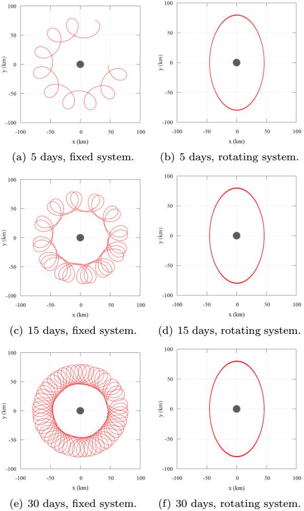
Fig. 7 Time evolution of trajectories obtained using Deimos at periapsis, D = 46.4 km, v x = 0, v y = −0.003 km/s, considering e = 0.0002, J 2 = 1960.45 × 10−6 for the simulation times 5, 15 and 30. The color figure can be viewed online.
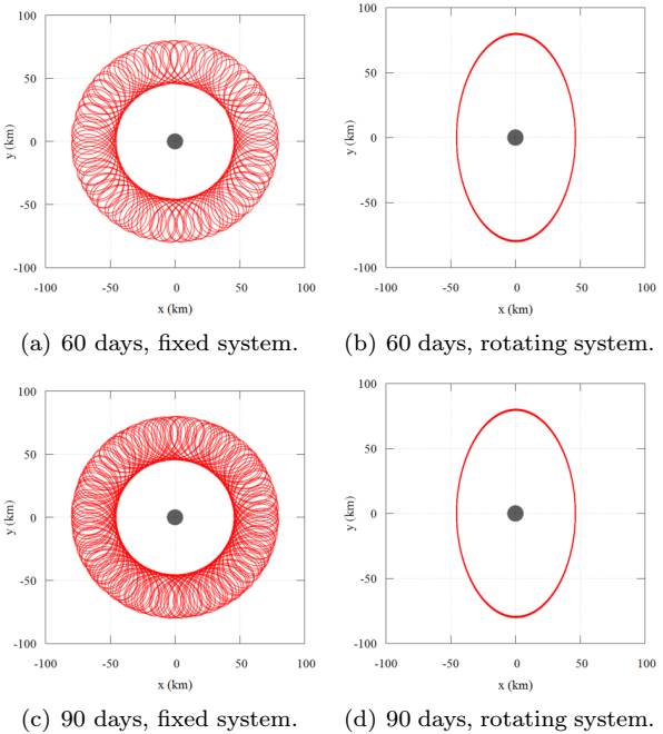
Fig. 8 Time evolution of trajectories obtained using Deimos at periapsis D = 46.4 km, v
x = 0, v
y= -003 km/s, considering e = 0.0002,
Now, we study this problem considering the initial position of Deimos at apoapsis. The results are shown in Figure 9 and Table 5. In Figure 9 the same set of initial conditions used to make Figures 2 and 3 is considered: the initial vertical component of the velocity v y is fixed in −0.003 km/s, the initial distance D ranges from 40 to 50 km and the horizontal component of the initial velocity ranges from −0.003 to 0.003 km/s. The maximum, minimum and average spacecraft-Deimos distances have a behavior similar to the one observed when Deimos is at periapsis. The lower values of D avg (Figure 9c), below 100 km, follow the smaller values of D max (Figure 9a), below 200 km, while the values of D min behave in an opposite way. However, the results with the lowest D max (Figure 9a) and D avg (Figure 9c) are shifted to the left with respect to Figures 2(a) and 2(c). This means that the initial position of Deimos influences the trajectories. For Figure 9, the lowest values of D max correspond to 31.03% of the total solutions, and the lowest values of D avg correspond to 17.52% of the total solutions. Comparing the lowest values of D max and D avg with those found when Deimos is at periapsis, 22.55% and 22.33%, respectively, there is an increase of 8.48% for D max and a decrease of 4.81% for D avg when Deimos is initially at apoapsis. The D max values, Figure 9(a), range from 75.93 to 23,534.69 km, that is, a range of values larger than the one found when Deimos is at periapsis, 80.24 to 22,330.45 km. The trajectory for the D max = 22,330.45 km is similar to the one shown in Figure 2, and the spacecraft goes away from Deimos to enter an orbit around Mars that is co-orbital with Deimos. The values of D min, Figure 9(b), range from 16.00 to 43.79, that is, a range of values larger than the one found when Deimos at periapsis, 16.00 to 45.43 km. The D avg values, Figure 9(c), range from 57.63 to 11,173.67 km, that is, a range of values larger than when Deimos is at periapsis, from 61.66 to 10,553.13 km. The values of D max and D avg are the most influenced by the position of Deimos, presenting smaller minimum values and larger maximum values when Deimos is at apoapsis. Figures 9(d), 9(e) and 9(f) show the results corresponding to Figures 9(a), 9(b) and 9(c), but now the model does not consider the effects of the flattening of Mars. The main difference is a slight reduction of the central blue region, which means that the maximum distances increase in this region. This happens for the maximum and average distances.
TABLE 5 THE FIVE ORBITS WITH SMALLEST D max (km) AROUND DEIMOS1
| D | vx | Davg | Dmin | Dmax | D∗avg | D∗min | D∗max | Davg −Davg ∗ | Dmin−D∗min | Dmax−D∗max |
|---|---|---|---|---|---|---|---|---|---|---|
| (km) | (km/s) | (km) | (km) | (km) | (km) | (km) | (km) | (km) | (km) | (km) |
| 43.8 | 0 | 61.1860 | 43.7992 | 75.9347 | 63.8417 | 43.8000 | 89.1615 | −2.6557 | −0.0008 | −13.2269 |
| 43.8 | −0.00001 | 61.1852 | 43.7469 | 76.2244 | 63.8406 | 43.7997 | 89.1683 | −2.6554 | −0.0527 | −12.9439 |
| 43.8 | 0.00001 | 61.1883 | 43.7472 | 76.2267 | 63.8440 | 43.8001 | 89.1563 | −2.6558 | −0.0529 | −12.9297 |
| 43.8 | −0.00002 | 61.1860 | 43.6957 | 76.5163 | 63.8408 | 43.7996 | 89.1749 | −2.6548 | −0.1039 | −12.6587 |
| 43.8 | 0.00002 | 61.1920 | 43.6923 | 76.5198 | 63.8477 | 43.7996 | 89.1558 | −2.6556 | −0.1073 | −12.63606 |
1Assuming vY = −0.003 km/s, Deimos initially at its apoapsis, e = 0.0002, J2 = 1960.45 × 10−6, T = 30 days.
Corresponding results for the circular and spherical model are represented by an asterisk (∗).
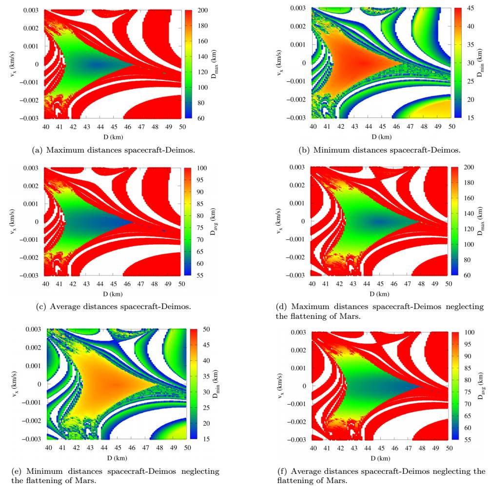
Fig. 9 Maximum, minimum and average spacecraft-Deimos distances, in km, as a function of D (km) and v x (km/s), considering v y = −0.003 km/s, for orbits with Deimos initially at apoapsis. The model considers e = 0.0002, J 2 = 1960.45 × 10−6, T = 30 days. The color figure can be viewed online.
Table 5 shows the five trajectories with the smallest values of D max, obtained with Deimos at apoapsis. The initial conditions have the values D = 43.8 km, v x = 0, ± 0.001 or 0.002 km/s and values of the maximum distances in the interval 75.90 to 76.50 km. In Table 2, Deimos is initially at periapsis, and the initial conditions were D = 46.30 or 46.40 km, v x = 0.000 or ±0.001 km/s and values of maximum distances in the interval from 80.20 to 80.30 km. Comparing the values shown in Tables 5 and 2, it is clear that the values of the initial distance D and the maximum distances are smaller when the moon is at apoapsis than when it is at periapsis.
Table 5 also shows that, when considering the simplest model (with circular orbits and a spherical shape for Mars) the differences for the minimum distance are between zero and 0.1 km; for the average distance they are around 2.65 km and for the maximum distance between 12.6 and 13.2 km, for an integration time of 30 days. The negative values of the last column of Table 5 imply that, when considering the simplest model, we overestimate D max. Comparing these results with those of Table 2, (for the periapsis case) it is observed that the values of the last column are of the order of 4 to 5 km, also negative, therefore smaller in magnitude than those presented in Table 5. This means that, when considering the simpler model in the apoapsis case, the values of the maximum distances are overestimated, as occurred in the periapsis case, but the errors are now about three times larger.
Figure 10 shows the trajectories with both models obtained with the data given by the first line of Table 5. The trajectories for the other lines of the table are very similar and they are omitted here. The left side considers the best model (elliptical orbit for Deimos and a flat body for Mars) and the right side the simplified model (circular orbit for Deimos and a spherical body for Mars). Note that the best model gives a near periodic orbit (but not periodic or quasiperiodic in terms of the known definitions), while the simple model gives an orbit with some oscillations in the spacecraft-Deimos distance.
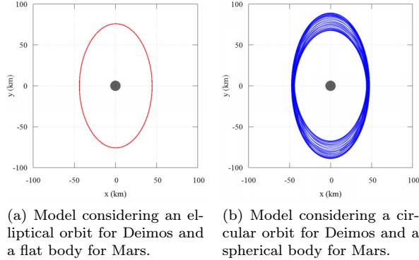
Fig. 10 Trajectories associated with the first line of Table 5 in the rotating frame. The color figure can be viewed online.
To conclude this study, the trajectory with the lowest D max from Table 5 is presented for T = 30 days in Figure 11. Deimos is plotted to scale and located at the origin. The values of distances (km) and disturbances (km/s2) for the time evolution of the trajectory at times 5, 10, 15, 30, 60, and 90 days are shown in Table 6. Figures 12 and 13 show the trajectory at the times shown in Table 6. Again, it is seen that the trajectory is quite stable in time, as in the periapsis case. In Figures 11(a) and 11(b) the full model is used, while in Figures 11(c) and 11(d) the simplest model is considered, assuming a circular orbit for Deimos and spherical shape for Mars. It is seen that the trajectory of the most complete model shows smaller oscillations than the trajectory of the simplest model. The minimum distances are very similar, but the maximum distances are much smaller for the more complete model (75.9347 against 89.1615 km). Many more regular orbits are generated by the best model.
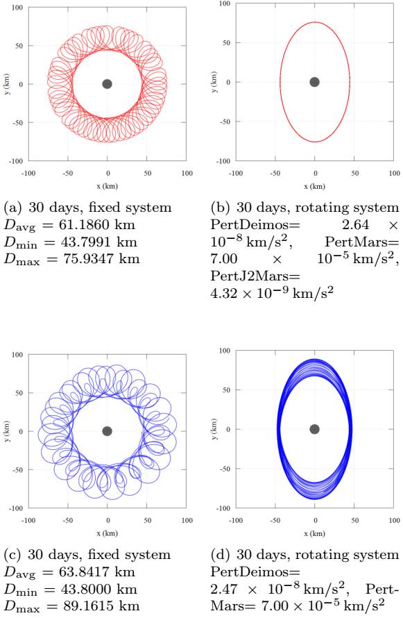
Fig. 11 Trajectories considering an elliptical orbit for Deimos and a flat body for Mars (red), and considering a circular orbit for Deimos and a spherical shape for Mars (blue). Deimos is initially at apoapsis, D = 43.8 km, v x = 0, v y = −0.003 km/s, T = 30 days. The color figure can be viewed online.
TABLE 6 DEIMOS AT APOAPSIS, D = 43.8 km, v x = 0 km/s, v y = −0.003 km/s*
|
|
|
|
|
|
|
|
|
|
|
|
|
|
|
|
|
|
|
|
|
|
|
|
|
|
|
|
| PertDeimos |
|
|
|
|
|
|
|
|||||
| PertMars |
|
|
|
|
|
|
|
|||||
| PertJ2Mars |
|
|
|
|
|
|
|
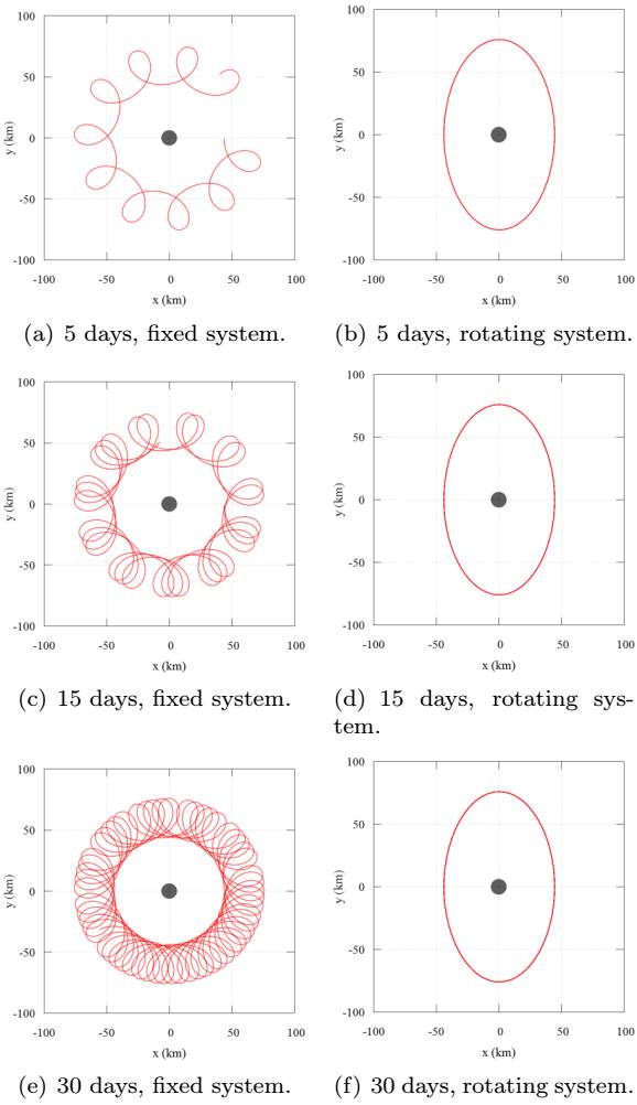
Fig. 12 Trajectories at times 5, 10, 15, and 30 days shown in Table 6. The color figure can be viewed online.
4. CONCLUSION
In this study a recently developed method for mapping orbits around small bodies was applied to Deimos, considering the maximum, minimum and average distances between Deimos and the spacecraft during a given time as the main criterion to select the orbits. The trajectories were mapped and plotted according to their initial conditions (position and velocity), to identify the conditions that keep the spacecraft at mid-range distances to Deimos, and to find orbits free from risks of collision but not too far away from Deimos. The method generated several results showing its efficiency in obtaining mid-range orbits around Deimos that are affected enough by the moon to keep the spacecraft near to it, although the orbit is really dominated by Mars.
The orbits found can be used to place a spacecraft as soon as it arrives in the vicinity of Deimos, to carry out the first detailed studies of the moon without having a large risk of collision. In this way, it is not necessary to know details about the shape of Deimos in advance. After more detailed studies made from these mid-range distances, the spacecraft can be placed in orbits closer to Deimos.
Among the many trajectories found, those that were considered good options are the ones that have Deimos-spacecraft distances in the range of 40 to 200 km over the 30 days of simulation. Using these trajectories, it is possible to make the first detailed observations of Deimos without the risk of collision with it. It was also shown that many of these trajectories are able to survive for up to 90 days and that the orbits are very regular, keeping about the same values of distances and perturbations levels over time.
The initial position of Deimos in its orbit around Mars showed effects on the behavior of the orbit. Depending on its initial condition there are differences in the values of maximum, minimum and average spacecraft-Deimos distances when considering the moon at periapsis or apoapsis. These two positions gave good options for trajectories, but the results found when Deimos is at apoapsis are better than the corresponding ones with Deimos at periapsis, because the maximum distances were smaller when at apoapsis than at periapsis.
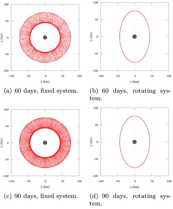
Fig. 13 Trajectories at times 60 and 90 days showed in Table 6. The color figure can be viewed online.
The importance of the mathematical model adopted was also shown by comparing it with a more complete model, which considers Deimos in an elliptic orbit around Mars and the J 2 term of the gravitational potential of Mars. The simplest model considered Deimos in a circular orbit and Mars as a spherical body. It was shown that, for the two positions of Deimos, periapsis and apoapsis, if the simplest model was adopted, the values of the maximum distances were overestimated with respect to the most complete model. With Deimos at periapsis these errors are of the order of 4-5 km, while they increase to around 12-13 km for Deimos at apoapsis.
The integrals of the accelerations of each force that acts in the spacecraft over time were also studied. Using this technique, it was possible to quantitatively measure the influence of each force acting in the dynamics of the system. It was shown that the results of the contribution of the gravitational interaction of Mars are about 3 orders of magnitude larger than the effects of the gravitational field of Deimos. This proves and quantifies that Mars is the body that dominates the motion of the spacecraft, while Deimos only disturbs this motion.

