


 text new page (beta)
 English (pdf)
 Article in xml format
 Article references
 Send this article by e-mail
 Cited by SciELO
  Similars in
SciELO
Similars in
SciELO 
 Permalink
1. INTRODUCTION
Infrared dark clouds (IRDCs) are sites of recent star formation within molecular clouds. These are detected as dark silhouettes against a bright background in the mid-infrared. These regions, which are also detected in the FIR, are believed to be places that may contain compact cores which probably host the early stages of high-mass star formation (e.g., Rathborne et al. 2007; Chambers et al. 2009). In fact, their cold (T < 25K) and dense (102-104 cm−3) ambient conditions, and their sizes of ≈1-3pc and masses of 102-104 M ⊙ (Rathborne et al. 2006, 2007) favor star formation mechanisms. Evidences of active high-mass star formation in IRDCs are inferred from the presence of ultracompact Hii regions (Battersby et al. 2010), hot cores (Rathborne et al. 2008), embedded 24µm sources (Chambers et al. 2009), maser emission (Wang et al. 2008; Chambers et al. 2009), and/or outflow and infall processes (e.g. Sanhueza et al. 2010; Chen et al. 2011; Ren et al. 2011; Beuther et al. 2002; Zhang et al. 2007).
Many IRDCs are also associated with extended enhanced 4.5 µm emission (named extended green objects, EGOs, for the common coding of the [4.5] band in green in the 3-color composite IRAC images), the so-called “green fuzzies”, indicating the presence of shocks. Following photometric criteria, Cyganowski et al. (2008) suggested that most of EGOs fall in the region of the color-color space occupied by the youngest MYSOs, and are surrounded by accreting envelopes (see Figure 13 in their work). This hypothesis is supported by Chen et al. (2010), whose observations are consistent with the speculation that EGOs trace a population with ongoing outflow activity and an active rapid accretion stage of massive protostellar evolution. The emission at 4.5µm includes both H2 (v = 0-0, S(9, 10, 11)) lines and CO (v = 1-0) band heads (Cyganowski et al. 2008), which are excited by shocks, such as those expected when protostellar outflows impinge on the ambient interstellar medium (ISM) (Cyganowski et al. 2008).
Using IRAC images, Peretto & Fuller (2009) catalogued and characterized many IRDCs using 8 and 24µm Spitzer data. In this catalogue, the IRDCs were defined as connected structures with H2 column density peaks N H2 > 2×1022 cm−2 and boundaries defined by N H2 = 1×1022 cm−2. Single-peaked structures found in the H2 column density maps were identified by the authors as fragments. These dark and dense patches are associated with molecular gas and dust emission (Sanhueza et al. 2012).
As a part of a project aimed at studying in detail the physical properties of the IR bubble complex S21-S24, we present here an analysis of the molecular gas and dust associated with SDC341.232-0.268, a poorly studied IRDC of the southern hemisphere, which is member of this complex. Our aims are to determine the physical parameters and kinematics of the gas and to characterize the interstellar dust associated with the IRDC, to investigate the presence of embedded young stellar objects, and to establish possible infall or outflow gas motions. To accomplish this project, we analyze molecular data of the 12CO(2-1), 13CO(2-1), and C18O(2-1) lines obtained with the APEX telescope, and HCO+(1-0), HNC(1-0), and N2H+(1-0) lines from the MALT90 survey (Jackson et al. 2013; Foster et al. 2013, 2011)7, mid- and far-IR continuum data from Spitzer-IRAC, Herschel-PACS and -SPIRE, and ATLASGAL (APEX) images (Schuller et al. 2009). We introduce the IRDC SDC341.232-0.268 in § 2, the used database in § 3, the results of the molecular gas in § 4, and those of the infrared emission in § 5; signs of star formation are discussed in § 6, and a summary in § 7.
2. IRDC SDC341.232-0.268
The IRDC SDC341.232-0.268 (RA,Dec.(J2000)= 16:52:35.67, -44:28:21.8) has a mid-IR radiation field intensity I MIR ≈ 88.3 MJy ster−1 at 8.0µm and a peak opacity of 1.09. From the Multiband Infrared Photometer for Spitzer (MIPS) images Peretto & Fuller (2009) detected a 24µm point source in the field of the IRDC, and two clumps. The clumps were classified by Bergin & Tafalla (2007) as structures with sizes ≈10−1-100 pc, masses ≈10-103 M ⊙, and volume densities ≈103-104 cm−3.
Figure 1 shows the Spitzer-IRAC images at 4.5 (green) and 8.0µm (red), and the Spitzer-MIPS image at 24µm (blue) in the region of SDC341.232-0.268. Green contours correspond to low emission levels at 8µm, revealing a region of high extinction at 8.0µm at the location of the IRDC, in contrast with the environment, a typical feature of these objects. The 90 MJy/ster contour delineates the IRDC. Four candidate EGOs catalogued by Cyganowski et al. (2008) appear projected toward this region: the “likely” MYSO outflow candidates G341.22-0.26(b)(R.A., Decl.(J2000) = 16:52:30.3, -44:28:40.0), G341.22-0.26(a) (16:52:32.2, -44:28:38.0), the “possible” MYSO outflow candidate G341.23-0.27 (16:52:34.2, -44:28:36.0), and the “likely” MYSO outflow candidate G341.24-0.27 (16:52:37.3, -44:28:09.0). These authors categorized the EGOs as a “likely” or “possible” MYSO outflow candidate based primarily on the angular extent of the extended excess 4.5 µm emission. Any source in which it was possible to confuse multiple nearby point sources and/or image artifacts from a bright IRAC with truly extended 4.5 µm emission was considered a “possible” candidate; these are likely still good YSO candidates, but not necessarily MYSOs with outflows, and so likely to be actively accreting.
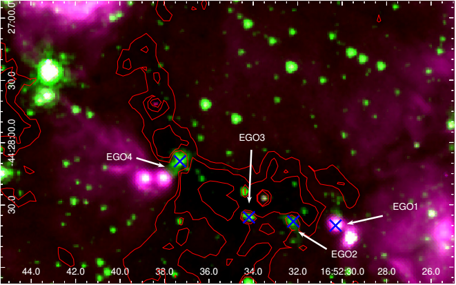
Fig. 1 Composite image showing the Spitzer-IRAC emission at 4.5 (green) and 8.0µm (red), and Spitzer-MIPS emission at 24µm (blue) of the region of SDC341.232-0.268. Contours correspond to the emission at 8.0µm at 80, 90, and 95 MJy/ster. The positions of the candidate EGOs are marked with blue crosses. The color figure can be viewed online.
From here on, they will be named EGO1, EGO2, EGO3, and EGO4, in increasing order of R.A. EGO1 is associated with 8 and 24µm emission and is located in the border of the IRDC, while EGOs 2, 3, and 4 are detected at 4.5 and 8µm. EGO1 and EGO4 coincide with ATLASGAL Compact Sources AGAL341.219-00.259 and AGAL341.236-00.271. Their integrated flux densities are 12.85±2.20 Jy and 16.81±2.80 Jy, and their effective radii are ≈ 37′′ and 47′′, respectively (Contreras et al. 2013).
Methanol maser emission was detected towards EGO2 and EGO4 at 6 and 95 GHz, within the velocity range −43 to −52km s−1(Caswell et al. 2010; Chen et al. 2011; Hou & Han 2014; Yang et al. 2017). Methanol masers provide a signpost to the very earliest stages of the massive star formation process, prior to the onset of the UCHII region phase. They are associated with embedded sources whose bolometric luminosities suggest that they will soon become OB stars (Burton et al. 2002; Sobolev et al. 2005). The methanol masers are independent tracers and they give proven signatures of ongoing star formation (see Ellingsen 2006; Breen et al. 2013). Masers of water or hydroxyl have also been detected in in star-forming regions, as well as in evolved stars or supernova remnants. Therefore, the presence of these maser types in the vicinity of these EGOs could be a signspot of ongoing star formation.
3. DATABASE
3.1. Molecular Line Observations
The 12CO(2-1), 13CO(2-1), and C18O(2-1) data were acquired with the APEX-1 receiver of the Swedish Heterodyne Facility Instrument (SHeFI; Vassilev et al. 2008) in the Atacama Pathfinder EXperiment (APEX) telescope, located in the Puna de Atacama (Chile). The backend for the observations was the eXtended bandwidth Fast Fourier Transform Spectrometer2 (XFFTS2) with a 2.5 GHz bandwidth divided into 32768 channels. The main parameters of the molecular transitions (rest frequency ν 0, halfpower beam-width θ, velocity resolution ∆vres, and rms noise of the individual spectra obtained using the OTF mode) are listed in Table 1. The selected off-source position free of molecular emission was RA, Dec.(J2000)= (16:36:40.56, −42:03:40.6).
TABLE 1 OBSERVATIONAL PARAMETERS OF THE MOLECULAR TRANSITIONS
| Transition | ν 0 | θ | ∆v res | rms |
|---|---|---|---|---|
| GHz | ′′ | km s−1 | K | |
| 12CO(2-1) | 230.538 | 30 | 0.1 | 0.35 |
| 13CO(2-1) | 220.398 | 28.5 | 0.1 | 0.35 |
| C18O(2-1) | 219.560 | 28.3 | 0.1 | 0.35 |
| HNC(1-0) | 90.664 | 38.0 | 0.11 | 0.35 |
| HCO+(1-0) | 89.189 | 38.0 | 0.11 | 0.35 |
| N2H+(1-0) | 93.173 | 38.0 | 0.11 | 0.35 |
Calibration was done using the chopper-wheel technique. The antenna temperature scale was converted to the main-beam brightness-temperature scale by T mb = T A/η mb, where η mb is the main beam efficiency. For the SHeFI/APEX-1 receiver we adopted η mb = 0.75. Ambient conditions were good, with a precipitable water vapor (PWV) between 1.5 - 2.0 mm.
The molecular spectra were reduced using the CLASS90 software of the IRAM’s GILDAS software package.
In addition, we used molecular data from the Millimetre Astronomy Legacy Team 90 GHz Survey (MALT90) taken with the Mopra spectrometer (MOPS). We used beam efficiencies between 0.49 at 86 GHz and 0.42 at 230GHz (Ladd et al. 2005). The data analysis was conducted with CLASS90 software. Emission was detected in the HCO+(1-0), HNC(1-0), and N2H+(1-0) lines, which were used to detect high density regions within SDC341.232-0.268. Their main parameters are included in Table 1.
3.2. Images in the Infrared
We used near- and mid-infrared (NIR, MIR) images from the Spitzer-IRAC archive at 4.5 and 8.0µm of the Galactic Legacy Infrared Mid-Plane Survey Extraordinaire (GLIMPSE)8 (Benjamin et al. 2003), and the Multiband Imaging Photometer for Spitzer (MIPS) image at 24µm from the MIPS Inner Galactic Plane Survey (MIPSGAL)9 (Carey et al. 2005) to delineate the IRDC and investigate their correlation with the EGO candidates.
To trace the cold dust emission we utilized farinfrared (FIR) images from the Herschel Space Observatory belonging to the Infrared GALactic (HiGAL) plane survey key program (Molinari et al. 2010). The data were obtained out in parallel mode with the instruments PACS (Poglitsch et al. 2010) at 70 and 160µm, and SPIRE (Griffin et al. 2010) at 250, 350, and 500µm. The angular resolutions for the five photometric bands spans from 8′′ to 35′′ .2 for 70µm to 500µm. Herschel Interactive Processing Environment (HIPE v1210, Ott 2010) was used to reduce the data, with reduction scripts from standard processing. The data reduction and calibration (including zero-level and color correction) is described in detail in § 2.2 of Cappa et al. (2016).
We also used images at 870µm from the APEX Telescope Large Area Survey of the Galaxy (ATLASGAL) (Schuller et al. 2009) with a beam size of 19′′ .2. This survey covers the inner Galactic plane, with an rms noise in the range 0.05-0.07 Jy beam−1. The calibration uncertainty in the final maps is about 15%.
4. MOLECULAR CHARACTERIZATION OFTHE IRDC
4.1. CO data: Morphological and Kinematical Description
To visualize the spatial distribution of the molecular emission the upper panel of Figure 2 exhibits the 13CO(2-1) brightness temperature distribution from ≈ −47.0 to −42.5 km s−1 in steps of 0.3 km s−1. The most intense 13CO(2-1) emission appears in the range −45.2 to −44 km s−1. The bottom central panel of Figure 2 shows the average 13CO(2-1) emission in the range −47.0 to −42.8 km s−1, revealing two molecular clumps centered at RA, Dec.(J2000)= (16:52:37.06, −44:28:13.9) (Clump A) and RA, Dec.(J2000)= (16:52:29.72, −44:28:40.1) (Clump B). The coincidence of the clumps with EGO1, 2, and 4 (indicated with crosses in this figure) is clear. The effective radii of the clumps are 37′′ .6 and 45′′ .6 for ClumpA and ClumpB, respectively, as obtained taking into account the average 13CO(2-1) emission higher that 6.2 K. Finally, the bottom left and right panels of the same figure display the C18O(2-1) and 12CO(2-1) average emission in velocity intervals similar to that in the image of 13CO(2-1). Both clumps A and B are detected at C18O(2-1) revealing the existence of dense molecular gas in the clumps. The 12CO(2-1) emission delineates the IRDC but the clumps are not well defined.
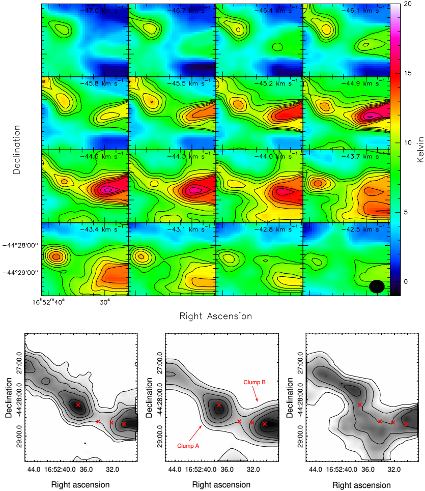
Fig. 2 Upper panel: T mb-maps of the 13CO(2-1) emission within the velocity interval from -47.0 to -42.5km s−1 in steps of 0.3km s−1. Contours range from 8 to 17K in steps of 1K in T mb. Lower left panel: Average C18O(2-1) emission in the range -47.2 to -43.8km s−1. Contours are 0.8, 1.0, 1.3, 1.6, and 2.0K. The red crosses mark the position of the EGOs. Lower central panel: Average 13CO(2-1) emission in the range −47.0 to −42.8km s−1. Contours range from 6.2 to 9.4K in steps of 0.8K. Lower right panel: Average 12CO(2-1) emission in the range −48.2 to −42.5km s−1. Contours range from 10 to 13K in steps of 1K. The color figure can be viewed online.
Figure 3 shows the averaged 12CO(2-1), 13CO(2-1), and C18O(2-1) spectra within the area corresponding to ClumpA and ClumpB. The rms noise of the averaged spectra is 0.019 K for ClumpA, and 0.017 for ClumpB. For ClumpA, the 12CO(2-1) line exhibits a multi-peak structure with components in the interval from −70 to −20 km s−1, with the most intense features between −48 and −35 km s−1. Three velocity componentes are detected within the latter velocity interval, peaking at −46.6 km s−1, −42.2 km s−1, and −36.8 km s−1. The 13CO(2-1) and C18O(2-1) spectra peak at around −44.0 km s−1, coincident with a minimum in the 12CO(2-1) spectrum. Components outside this range will be analyzed in § 6.2. For ClumpB, the 12CO(2-1) line also shows a multi-peak structure between -55 and -25 km s−1, with the maximum at -45.4 km s−1. The 13CO(2-1) and C18O(2-1) profiles peak at -44.0 km s−1.

Taking into account that the C18O(2-1) emission is generally optically thin, we adopted systemic velocities (v sys) of -44.0 km s−1 for ClumpA and ClumpB. The adopted systemic velocity coincides with the velocity for EGO2 and 4 reported by Yang et al. (2017) (−44.6 and −44.9, respectively) from methanol maser emision, and from masers by Chen et al. (2011). It is also compatible with the velocity of NH3 clouds identified by Purcell et al. (2012) at −43.7 km s−1 at a position distant 15′′ from EGO3, and from the CS(2-1) line emission obtained by Bronfman et al. (1996), who observed toward [RA, Dec.(J2000)= (16:52:34.2, -44:28:36.0)], revealing the presence of high density regions (n crit = 3.0 × 105 cm−3). Circular galactic rotation models predict that gas with velocities of −44 km s−1 lies at the near kinematical distance of 3.6 kpc (see, for example, Brand & Blitz 1993). Adopting a velocity dispersion of 6km s−1, the uncertainty in distance is 0.5kpc (15%). The distance coincides also with that of S24 (Cappa et al. 2016) indicating that the IRDC belongs to the same complex.
TABLE 2 PARAMETERS OF THE GAUSSIAN FITS FOR ClumpA AND ClumpB
| Line | v | ∆v | T peak | Area | |
|---|---|---|---|---|---|
| km s−1 | km s−1 | K | K km s−1 | ||
| Clump A | CO(2-1) | -44.56(0.03) | 5.56(0.07) | 6.82 | 40.33(0.41) |
| C18O(2-1) | -44.23(0.02) | 4.46(0.05) | 1.37 | 6.49(0.06) | |
| Clump B | 13CO(2-1) C18O(2-1) | -43.85(0.01) -43.70(0.01) | 2.56(0.08) 2.61(0.03) | 9.52 2.46 | 25.96(0.18) 6.84(0.07) |
4.2. Parameters Derived From CO Data
Bearing in mind that the spatial distribution of the 13CO(2-1) and C18O(2-1) emission coincides with the IRDC, we used these lines to estimate the main parameters of the molecular gas assuming local thermodynamic equilibrium (LTE). All the calculations were carried out from the Gaussian fits to the lines averaged in the area of ClumpA and ClumpB shown in Table 2. The columns list the central velocity of each component v, the full-width at halfmaximum, the peak temperature, and the integrated emission. We applied the following expression to estimate optical depths (e.g. Scoville et al. 1986):
where τ 13 is the optical depth of the 13CO(2-1) gas and 7.6 = [13CO(2-1)]/[C18O(2-1)] (Sanhueza et al. 2010) is the isotope abundance ratio. The 13CO(2-1) optical depths are indicated in Column 2 of Table 3. To estimate the C18O(2-1) optical depth we used
where ∆v is the full-width at half-maximum of the C18O(2-1) and 13CO(2-1) profiles. The results are listed in Column 3 of Table 3. Bearing in mind that 13CO(2-1) is moderately optically thick we calculated the excitation temperature from the 13CO(2-1) line using
where
The column density for 13CO(2-1) was derived using Rohlfs & Wilson (2004)
In this case we used the approximation for τ 13 > 1,
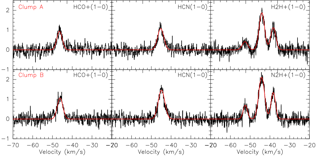
Fig. 4 HCO+(1-0), HNC(1-0) and N2H+(1-0) profiles towards ClumpA (top) and ClumpB (bottom). The color figure can be viewed online.
This approximation helps to eliminate to some extent optical depth effects. The integral was evaluated as T mean − mb ×∆v, where T mean − mb is equal to the average T mb within the area of each clump.
To estimate N(H2) (Column 6 in Table 3) we adopted an abundance [H2][13CO]= 5×10⁵ (Dickman 1978). Then, the molecular mass (Column 9 in Table 3) was calculated from the equation
where m sun = 2×1033 g is the solar mass, the mean molecular weight µ = 2.76 (which includes a relative helium abundance of 25% by mass, Allen 1973), and m H is the hydrogen atomic mass. In this expression d is the distance, N(H 2) is the H2 column density, and A is the area of the source in cm−2. The effective radius of each clump, as seen in the 13CO(2-1) line, and the volume densities are listed in Colums 7 and 9 in Table 3.
The ambient volume densities, n H2, was calculated assuming a spherical geometry for the clumps, using the formula
Ambient densities are listed in Column 9 of Table 3. The parameters calculated in this work agree with Bergin & Tafalla (2007).
The virial mass can be determined following MacLaren et al. (1988):
where r and ∆v are the radius of the region and the velocity width measured from the Gaussian fit of the C18O(2-1) emission, and k 2 depends on the geometry of the ambient gas in the region, being 190 or 126 according to ρ ∝ r −1 or ρ ∝ r −2, respectively. M vir values are listed in Column 10 in Table 3. The ratios M vir /M(H 2) suggest that both clumps may collapse to form new stars; since the virial mass value is smaller than the LTE mass value this clump does not have enough kinetic energy to stop the gravitational collapse.
Uncertainties in both the molecular mass derived using LTE conditions, M(H2), and the virial mass M vir are affected by the distance indetermination (15%) yielding a 30% error in M(H2) and 15% in M vir. Inaccuracies in the borders of the clumps originate errors in their sizes and thus additional uncertainties in the masses, suggesting errors of 40% in M(H2). Virial masses are not free of uncertainties, because of the existence of magnetic field support that may lead to an overestimate of the derived values (see MacLaren et al. 1988), and because of the unknown density profile of the clump.
4.2.1. Analysis of the MALT90 Data
The MALT90 data cubes of this region show emission of HCO+(1-0), HNC(1-0), and N2H+(1-0) molecules, which are the most often detected molecules towards IRDCs (Sanhueza et al. 2012; Rathborne et al. 2016). These molecules have critical densities of 2×10⁵, 3×10⁵ and 3×105 cm−3, respectively (Sanhueza et al. 2012), allowing us to infer a lower limit for the density of the clumps. These values are higher than the H2 ambient densities derived from CO lines (see Table 3).
Spectra of these lines, averaged over the area of the clumps, are shown in Figure 5. By applying a Gaussian fitting to the HCO+ and HNC lines, a mean velocity of −46 km s−1 was derived. For the case of the N2H+ line, a multi Gaussian function was applied to take into account hyperfine structure. This molecule has seven hyperfine components in two blended groups of three lines (groups 2 and 3) and one isolated component (group 1). The rest frequencies of groups 1, 2 and 3 are 93.176, 93.173, and 93.171 GHz, respectively. The mean velocity is −44 km s−1. The velocities of these lines coincide with the systemic velocities derived from CO data.

Fig. 5 HCO+(1-0) (levs: 0.65, 0.7, 0.8 and 0.9 K), HNC(1-0) (levs: 0.7, 0.85, 1.0 and 1.15 K) and N2H+(1-0) (levs: 0.8, 1.0, 1.2 and 1.4 K) maps. Red circles have radii equal to the effective radii of the clumps as seen in 13CO(2-1), and are located at their position. Crosses mark the location of the EGO candidates. The color figure can be viewed online.
These tracers of dense gas provide slightly different information: HCO+ often shows infall signatures and outflow wings (e.g. Rawlings et al. 2004; Fuller et al. 2005). However, in our case no signs of infall can be identified. HNC is specially preponderant in cold gas and is a commonly used tracer of dense gas in molecular clouds. Finally, N2H+ is more resistant to freeze-out on grains than carbon-bearing species like CO.
Figure 5 shows the HCO+(1-0), HNC(1-0) and N2H+(1-0) maps, integrated from −47.6 to −44.0 km s−1, −46.7 to −43.1 km s−1, and −47 to −41.4 km s−1, respectively. Both clumps are detected in the three molecular lines indicating mean densities of 105 cm−3. Carbon-bearing species, like CO, tend to disappear from the gas phase in the high density centers of the cores, while nitrogen-bearing species like N2H+ survive almost unaffected up to much higher densities. This is evidenced in the fact that the spacial distribution of the N2H+ emission is similar to that of dust continuum emission (see Figure 6).

Fig. 6 FIR view of SDC341.232-0.268 from Herschel (70-500µm) and ATLASGAL data. The blue circles have the same meaning as in Figure 5 and show the areas where the flux densities were integrated. The crosses mark the position of the EGOs. Contours correspond to 20rms. The color figure can be viewed online.
Following Purcell et al. (2009) we estimate the N2H+ optical depth and column density. Assuming the line widths of the individual hyperfine components are all equal, the integrated intensities of the three blended groups should be in the ratio of 1:5:3 under optically thin conditions. The optical depth can then be derived from the ratio of the integrated intensities of any group using the following equation:
where a is the expected ratio of τ 1 /τ 2 under optically thin conditions.
To determine the optical depth we used only the intensity ratio of group 1/group 2, as Caselli et al. (1995) report anomalous excitation of the F1,F = 1,0 → 1,1 and 1,2 → 1,2 components (in group 3). Thus we obtained τ 1 = 0.11 and 0.19 for ClumpA and ClumpB, respectively.
Based on the expression for T mb given by Rohlfs & Wilson (2004), the excitation temperature for N2H+ can be calculated with the following formula:
and the column densities can be derived using (Chen et al. 2013):
where k is the Boltzmann constant, W is the observed line integrated intensity (obtained from a Gaussian fit), ν is the frequency of the transition, and Sµ 2 is the product of the total torsion-rotational line strength and the square of the electric dipole moment. T exc and T bg are the excitation temperature and background brightness temperature, respectively. E u /k is the upper level energy in K, Q(T exc) is the partition function at temperature T exc and τ is the optical depth. For group 1 the values of ν, Sµ 2 and E u /k are 93176.2526 MHz, 12.42D2 and 4.47K, respectively. These values were taken from the SPLATALOGUE catalogue11.
We derive T exc = 17.4 and 12.5K, and N(N2H+) = 8.7×10¹³ and 8.1×10¹³ for ClumpA and ClumpB, respectively. Considering an abundance [N2H+]/[H2] = 5×10⁻¹⁰ for dark molecular clouds (Ohishi et al. 1992) we obtain H2 column densities of 1.7 and 1.6 ×10²³ for ClumpA and ClumpB, respectively. These column densities are higher than those obtained from CO calculations. Ambient densities are n H2 ≈ 1.7×105 cm−3 for each clump with an effective radii in N2H+ of 0.53pc. This difference may be explained by considering that the nitrogen-bearing species survive almost unaffected up to much larger densities that carbon-bearing molecules.
5. WARM AND COLD DUST DISTRIBUTION
Figure 6 shows Herschel and ATLASGAL maps (in original resolution) of the SDC341.232-0.268 region. At λ < 160 µm the beam resolution allows to identify the emission associated with EGOs 1, 2, and 4. Warm dust coincident with the EGOs is also revealed by the emission in 24µm, which can be seen in Figure 1. The presence of this emission allows us to classify the clumps as “active”, according to the classification of Chambers et al. (2009). These authors proposed an evolutionary sequence in which “quiescent” clumps (containing neither IR indicator) evolve into “intermediate” (containing either a “green fuzzy” or a 24 µm point source, but not both), “active”(caracterized by the presence of a “green fuzzy” coincident with an embedded 24µm source, such as those observed toward EGOs 1, 2, and 4), and “red” clumps (dominated by 8 µm emission, which contains PAH features). At λ > 160µm two dust clumps are detected superimposed onto more extended submillimeter emission, indicating dust related to ClumpA and ClumpB.
The characterization of the dust properties of these clumps is limited by the resolution of FIR data. We study the integrated dust properties of each clump from the spectral energy distribution (SED) using the Herschel (160 up to 500 µm) and ATLASGAL maps convolved at a common beam resolution of the 500 µm map (36′′). The flux densities are obtained from a circular aperture photometry integration (radius of 37′′ .6 and 45′′ .6 for ClumpA and ClumpB, respectively), and subtracting a background level computed from a rectangular region (width = 52′′ .5 and height 25′′ .8 in the north of the clumps). For flux uncertainty estimation, we consider the standard deviation of surface brightness in the background region and the flux calibration uncertainties. For each clumps, the final SED is depicted in Figure 7 and the fluxes and their error bars are listed in Table 4. We perform a thermal dust fit to the data considering a single-component modified blackbody (grey-boby), which depends on the optical depth, the emissivity spectral index (β d ) and the dust temperature (T d ). In the optically thin regime, the best fitting provides similar dust temperature and emissivity for both clumps, with values of T d = 13.5 ± 0.47 K and β d = 2.7. These dust temperatures are of the order of those found by Guzmán et al. (2015) (18.6±0.2) for proto-stellar clumps.

Fig. 7 Spectral energy distributions (SEDs) for ClumpA (left) and ClumpB (right), obtained from the fluxes at 160, 250, 350, and 500µm from Herschel, and 870µm from ATLASGAL. The color figure can be viewed online.
TABLE 4 MEASURED FLUXES AND DERIVED PARAMETERS OF THE FIR CLUMPS
| S160 | S250 | S350 | S500 | S870 | T d | M dust+gas | nH2 | |
|---|---|---|---|---|---|---|---|---|
| [Jy] | [Jy] | [Jy] | [Jy] | [Jy] | [K] | [ |
[103 cm−3] | |
| ClumpA | 293±53 | 281±21 | 151±8 | 56±3 | 5.2±0.4 | 13.6±0.47 | 1536±444 | 1.5±0.7 |
| ClumpB | 421±53 | 376±21 | 195±8 | 74±3 | 6.3±0.6 | 13.5±0.47 | 2088±600 | 1.4±0.6 |
For ClumpA and ClumpB, the total mass(M dust+gas) was calculated from the optical depth of the dust obtained from the fit, using the following expression
whereτ νfit is the dust optical depth (= 10−26× fit amplitude), ν fit =1Hz is the frequency of the fit, R d = 100 is the typical gas-to-dust ratio, d is the distance and κ 870=1.00 cm−2 gr−1 is the dust opacity at 345GHz (Ossenkopf & Henning 1994). The mass uncertainties were computed propagating the error bars for dust optical depth and distance. Additional errors may result from taking different values for the gas-to-dust ratio (in our galaxy typical values are between 100 and 150).
The results are listed in Table 4, which includes the derived masses of the clumps and their volume densities. Uncertainties in masses and ambient densities are about 35% and 60%, respectively. The total masses derived from molecular gas and dust emission are in good agrement (within errors).
6. STAR FORMATION
6.1. Search for Additional YSOs Coincident with the IRDC
To investigate the coincidence of the IRDC with other candidate young stellar objects (YSOs), we analyze the characteristics of the point sources in the WISE and Spitzer catalogues (Wright et al. 2010; Benjamin et al. 2003) projected in the region. In Figure 8 we mark the positions of Class I and II YSO candidates identified in the area of the molecular clumps. An inspection of the figure reveals that EGOs 1, 3, and 4 coincide with identified YSOs.
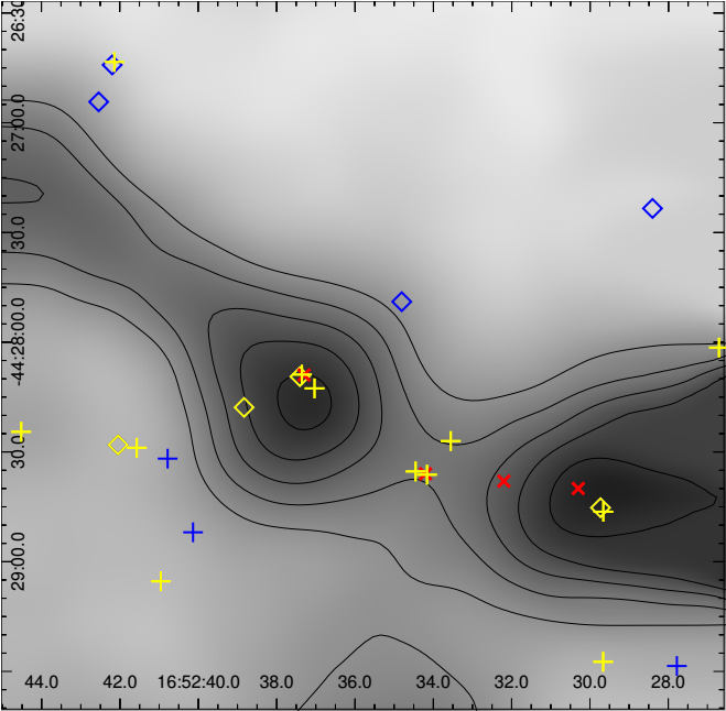
Fig. 8 Overlay of YSOs identified in the Spitzer and WISE catalogues and the molecular clumps in 13CO(2-1). Contours have the same meaning as in Figure 2. Yellow and blue symbols show the position of Class I and Class II YSOs, while red crosses mark the location of EGOs. Plus signs correspond to Spitzer sources and diamonds to WISE ones. The color figure can be viewed online.
To study in some detail the nature of the EGOs we plotted their spectral energy distributions (SEDs) using the Robitaille’s SED fitting tool (Robitaille et al. 2007). To perform the analysis we were able to use available data from 2MASS, IRAC-GLIMPSE, and MIPSGAL at 24µm only. The obtained SEDs are shown in Figure 9. Clearly, EGO 1, 3 and 4 have characteristics of YSOs, and as seen in Figure 8 coincide with additional evidence of star formation. As regards EGO2, the fit is not good; it does not coincide with other sources or with the molecular clumps. So, its status is doubtful. In Table 5 we display the main parameters obtained from the SEDs. Column 1 gives the name of the source; Columns 2 and 3, the age and mass, M stellar, of the central source; Column 4, the mass of the envelope, M env; Column 5, the infall rate, Ṁ acr; and Column 6, the total luminosity. To perform the SEDs we adopted d = 3.6±0.5 kpc and a visual extinction of 3-4 mag.
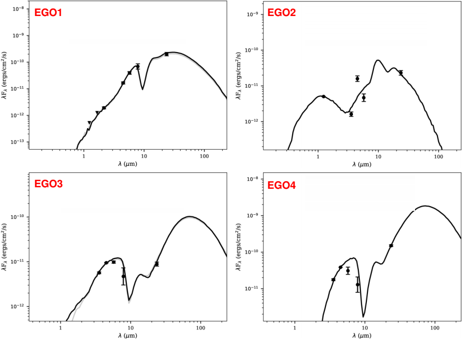
Fig. 9 Spectral energy distribution for the four candidate EGOs. The color figure can be viewed online.
TABLE 5 PHYSICAL PARAMETERS OBTAINED FROM THE SEDS FOR THE EGOS
| Age |
|
|
|
|
Stage | |
|---|---|---|---|---|---|---|
| 10 |
M |
M |
10-4
|
102
|
||
| EGO 1 | 0.13 | 2.1 | 0.7 | 0.1 | 1.3 | 0/I |
| EGO 2 | 545 | 3.9 | 8 |
0 | 1.9 | 0/I |
| EGO 3 | 15.7 | 4.1 | 7.1 | 1.4 | 0.8 | 0/I |
| EGO 4 | 4.1 | 8.6 | 0.09 | 12.5 | 14.4 | 0/I |
Following Robitaille et al. (2007) an estimate of the evolutionary stage of the sources can be obtained based on the ratio of the infall rate and the mass of the central source. For the four candidate EGOs the ratio Ṁ acr /M stellar > 10−6 indicates Stage 0/I. The age of some of the sources suggests that they are still immersed in their envelopes. According to the fitting, EGO4 would be the most massive object in the sample, and EGO2 seems to be the most evolved one. These results should be taken with caution because of the limitations of the fitting tool that may arise from: (1) YSOs are complex 3d objects with slightly non-axisymmetric density structures, so the models are incorrect compared to actual density distributions; (2) there are often mixtures of sources and many objects appear as a single YSO, but they are often two or more objects; and (3) even in the case of an isolated YSO variability is an additional complication, since the data with which SEDs are usually constructed belong to different surveys that have been performed in different years and can produce discontinuities in the SEDs (Robitaille 2008; Deharveng et al. 2012; Offner et al. 2012).
As pointed out before, the emission at 24µm, detected toward EGO1, 3, and 4, suggests the existence of warm dust and embedded protostars (Jackson et al. 2008).
6.2. Evidence for Inflow/Outflow Motions
One way to visualize molecular outflows or infalls is to compare the optically thick 12CO(2-1) emission line with the optically thin C18O(2-1) molecular line toward the candidate EGOs, as shown in Figure 10 for EGO3 and EGO4. The 12CO(2-1) line presents a double peak structure with the blue shifted peak brighter than the red-shifted one, and a minimum at the systemic velocity, while the C18O(2-1) line presents a single peak centered on the absorption dip of the optically thick line. According to Chen et al. (2011) these spectra display characteristics typical of infall motions: a double-peak structure with the blue-shifted peak brighter than the red-shifted one, while an emission peak of an optically thin line appears centered on the absorption dip of the optically thick line. According to these authors, the infall motion is the only process that would consistently produce the blue profile asymmetry. The blue-shifted emission can be explained as due to high-excitation approaching warm gas located on the far side of the center of contraction. The emission of this gas undergoes less extinction than the emission from the red-shifted receding nearside material, given that the excitation temperature of the molecules increases toward the center of the region (Zhou 1992). Thus, the spectra of EGO3 and EGO4 suggest the presence of infall motions.
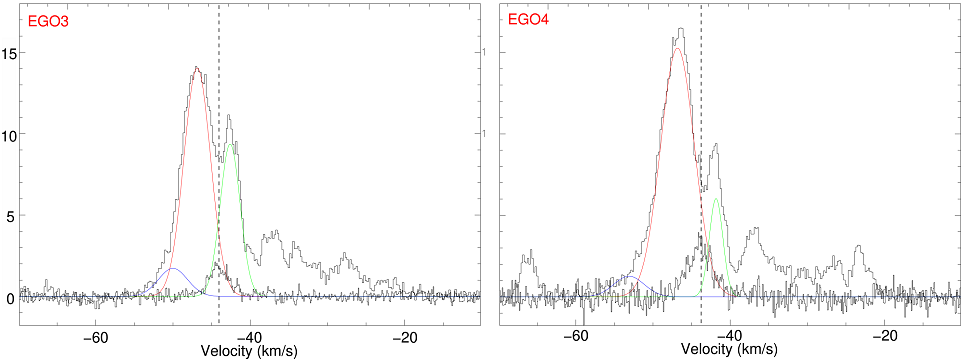
Fig. 10 12CO(2-1) and C18O(2-1) profiles in the direction to EGO3 (left) and EGO4 (right). In both pannels red and green lines correspond with Gaussian fits from the 12CO(2-1) double peak, and blue lines indicates a Gaussian component fitting the possible blue outflow wings. The color figure can be viewed online.
Following Mardones et al. (1997), we use the asymmetry parameter δv (the velocity difference between the peaks of the optically thick line and the optically thin lines, normalized by the FWHM of the thin line), to quantify the blue asymmetry. The parameter is defined as δv = (vthick - vthin) / ∆vthin. A statistically significant excess of blue asymmetric line profiles with δv < -0.25 indicates that the molecular gas is falling into the clump. We consider the velocity and width of the C18O(2-1), from Table 2, as vthin and ∆vthin, and calculate vthick from the Gaussian fits of 12CO(2-1) profiles (-46.9 and -45.3 from ClumpA and ClumpB, respectively). We find, for both ClumpA and ClumpB δv ≈ -0.06, which supports the infall hypothesis.
The interpretation presented above is supported by the M vir /M(H2) ratio previously derived for the objects. As the classical virial equilibrium análisis establishes, a ratio M vir /M(H2) < ∼ 1 indicates that a clump has too much kinetic energy and is unstable against gravitational collapse. Then, the derived ratios suggest that ClumpA and ClumpB are unstable and could be collapsing.
For the sake of completeness, we calculate the eventual infall rate estimated from Klaassen & Wilson (2007)
where n H2 is the H2 volume density, r clump is the linear radius of the infall region, and vinf is the infall velocity of the material. One way to estimate the infall velocity is considering the two layer radiative transfer model of Myers et al. (1996). From the 12CO(2-1) and C18O(2-1) spectra corresponding to ClumpA in Figure 3, we calculated vinf = 0.53 km s−1 using equation (9) in Myers et al. (1996). In order to get a better estimate, we also calculated the infall velocity using the Hill5 model (De Vries & Myers 2005) in the PySpecKit package (Ginsburg & Mirocha 2011) 12. The Hill5 model employs an excitation temperature profile increasing linearly toward the center, rather than the two-slab model of Myers et al. (1996), so the Hill5 model is thought to provide a better fit to infall motions (De Vries & Myers 2005). From this model we obtained vinf = 1.53 ± 0.26 km s−1. Considering this value of vinf = and the parameters listed in Table 3, we obtained Ṁ inf ≈ 7.47×10⁻⁴ M ⊙ yr−1. This result is consistent with those derived from surveys of massive YSOs such as Klaassen & Wilson (2007). ClumpB does not show clear observational evidences of collapse.
A typical outflow appears as spatially confined wings beyond the emission from the cloud core. For EGO3 and EGO4, we can distinguish the presence of 12CO(2-1) blue wings from ≈ -60 to -50 km s−1, shown in the spectra fit in Figure 10, while the velocity range of the optically thin C18O(2-1) emission is ≈ -47 to -40 km s−1. The dashed line marks the systemic velocity of the clumps, which coincides with the central velocity of the C18O(2-1) line. Red wings cannot be identified, although multiple components in the 12CO(2-1) emission are present.
The typical signature of outflows can be seen in the position-velocity diagram. As shown in Figure 11 for EGO4, the extension of the emission toward velocities of about -55 km s−1would correspond to the blue wings shown in Figure 10. Note that the declination of this extension and the right ascension of the map coincide with the position of EGO4.

Fig. 11 Position-velocity diagram toward EGO4 in 12CO(2-1) (Dec. vs. velocity for a fixed value of R.A. = 16:52:35). The color scale indicates Tmb and the declination is indicated in fractions of degrees. The color figure can be viewed online.
These characteristics suggest that, although they are not spatially resolved, there may be outflows associated with EGO3 and EGO4.
7. SUMMARY
Based on 12CO(2-1), 13CO(2-1), and C18O(2-1) images obtained using the APEX telescope and high density molecular tracers from the MALT90 survey such as HCO+(1-0), HNC(1-0) and N2H+(1-0) we investigate the molecular component of the IRDC SDC341.232-0.268. The 13CO(2-1) and C18O(2-1) along with MALT90 data reveal two molecular clumps (ClumpA and ClumpB) linked to SDC341.232-0.268 with systemic velocities of −44.0km s−1, indicating a kinematical distance of 3.6±0.5kpc. Four EGOs (EGO1 at RA,Dec = 16:52:30.3, −44:28:40.0; EGO2 at RA,Dec =16:52:32.2, −44:28:38.0; EGO3 at RA,Dec = 16:52:34.2, −44:28:36.0 and EGO4 at RA,Dec = 16:52:37.3, −44:28:09.9) coincide with the molecular clumps. We calculate masses of 2400±960 and 1200±480M ⊙, for ClumpA and ClumpB, respectively, and H2 ambient densities >104 cm−3. Ambient densities estimated using the N2H+(1-0) line are higher (≈ 105 cm−3) and agree with the critical density of this molecule, which would be tracing the densest part of the clumps.
Both ClumpA and ClumpB are detected in the FIR (Herschel images) at λ > 160µm. In the NIR and MIR, at λ < 160µm (24 and 70µm), three out of four EGOs seem to be resolved mainly at 24µm. Molecular masses derived from the emission at 870µm are roughly in agreement with those calculated from the molecular lines.
Spectral energy distributions (SEDs) for ClumpA and ClumpB built using fluxes in the FIR indicate dust temperatures of 13.5K, typical for an IRDC.
Our search for additional signs of star formation indicates that some of the EGOs coincides with young stellar objects classified as Class I detected as point sources in the Spitzer and WISE catalogs.
Additionally, the 12CO(2-1) spectra toward EGO3 and EGO4 present a double-peak structure with the blue-shifted peak brighter than the redshifted one, and with the maximum in the 13CO(2-1) and C18O(2-1) spectra coincident with the absorption dip, which reveals the existence of infall material. This fact together with the values obtained from M vir /M(H2) ratio derived for the clumps reveal that they would be collapsing. Blue extended wings in the C18O(2-1) spectra are also present toward these EGOs, suggesting the presence of outflows.

