


 nova página do texto(beta)
 Inglês (pdf)
 Artigo em XML
 Referências do artigo
 Enviar este artigo por email
 Citado por SciELO
  Similares em
SciELO
Similares em
SciELO 
 Permalink
1. Introduction
Recently, Maeder (2017a) proposed that the accelerating expansion of the Universe (Riess et al. 1998; Permultter et al. 1999) may be explained by the scale invariance of the empty space. It was argued that in empty space there is no preferred scale of length or time. He applied the theoretical framework developed for a scale-invariant theory of gravitation (Weyl 1923; Eddington 1923; Dirac 1973; Canuto et al. 1977) and found, as a result, that the effects of scale invariance are smaller when there is a greater quantity of matter present in the Universe.
This model has some interesting consequences. The cosmological constant, for example, is replaced by a variable term involving the scale-invariant scale factor. There is no need for a cosmological constant nor for dark energy in this context. The scale-invariant effects over the CMB temperature TCM B (z) were analysed by Maeder (2017b), where he found that if galactic corrections are applied, scale invariance may not be discarded. By analysing the Milky Way rotation curve in the context of scale invariant model, Maeder (2017c) argued that the flat rotation curves may be seen as an age effect and indicated that no dark matter was needed in this theoretical context.
This paper is focused on finding exact solutions of his equation of cosmological dynamics. Exact solutions provide transparency for the cosmological equations, may provide insights and can be used for a faster determination of cosmological constraints.
In
2. Scale-invariant cosmology
Maeder (2017a) shows that the general relativity (GR) metric is related to the scale-invariant one by
where c is the speed of light, which will be assumed to be unity elsewhere.
By applying the Robertson-Walker metric to a Universe filled with pressureless matter, he finds for the scale-invariant cosmology:
where R is the scale factor, time is expressed in units of t
0
= 1, k is the curvature constant, which can be 0, −1 or +1 for a spatially flat, open or closed Universe, respectively,
such that the normalization condition:
is valid.
Our focus here is to find exact solutions of (2). As nonflat exact solutions could not be found, we aim to solve the case where k = 0.
3. Flat scale-invariant cosmology
For the spatially flat Universe, the equation for scale-invariant Universe evolution (2)
where the time is expressed in units of t
0
= 1, and it is assumed that R
0
= 1. By evaluating (5) today, the relation for the Hubble constant
In order to solve (5), we replace R(t) by R(t) = tv(t), so:
and (5) may be written as:
So, we have to choose a sign for
In such a way that we have
where c 1 is an integration constant. From (9), we find
We want to solve (9) for v(t) in order to write R(t). We write v 3/2 = c 1 t 3/2 − v3 + C and square both sides. The result is:
Before writing the power as 2/3 in (11), there was an ambiguity sign inside the parentheses after we squared the expression (9). We must choose the sign which is in agreement with the initial condition (10). By choosing the negative sign inside the parentheses, we find
Now:
where we have replaced the value of c
1. As explained by Maeder (2017a) and shown in equations (3)-(4), in a flat scale invariant cosmology,
then
In Figure 1 we show some evolutions of the scale factor for different values of the density parameter, based on equation (15). It may be compared with Figure 2 of (Maeder 2017a), where the solutions were numerically obtained. No difference may be found between the exact and the numerical results.
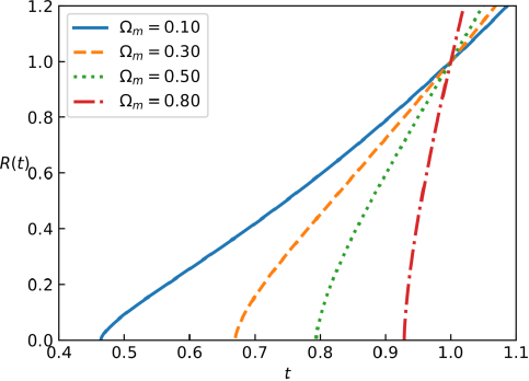
Fig. 1 Scale factor R(T) for some values of the matter density parameter in the flat scale-invariant cosmology. The color figure can be viewed online.
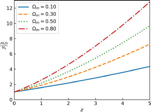
Fig. 2 Hubble parameter H(Z) for some values of the matter density parameter in the flat scale-invariant cosmology. The color figure can be viewed online.
As can be seen in Figure 1 and equation (15), with time in units of t 0 there is an initial time, t in, where R = 0. From (15), this time is:
From this we may write for the total age of the Universe,
By solving (15) for time, we may write for the age at redshift
Calculating
We solve equation (15) for time, then replace in (19) to find:
or, in terms of redshift z:
In Figure 2 is plotted H(z) for some values of the matter density parameter from equation (21).
From equations (15), (18) and (21) the results of Tables 1 and 2 of Maeder (2017a) can be recovered. No difference between analytical and numerical results could be found.
4. Conclusion
An interesting theory of scale-invariant cosmology was recently proposed. While the original focus was on the numerics, here we focus on finding an exact solution, at least for the spatially flat case. We show that our exact solution does not deviate from the original numerical solution. Physical insights about the dynamical equations may now be developed and cosmological constraints can be obtained faster.
JFJ is supported by Fundação de Amparo à Pesquisa do Estado de São Paulo - FAPESP (Process no. 2017/05859-0).

