


 text new page (beta)
 English (pdf)
 Article in xml format
 Article references
 Send this article by e-mail
 Cited by SciELO
  Similars in
SciELO
Similars in
SciELO 
 Permalink
1. INTRODUCTION
Cataclysmic variable stars (CVs) are semi-detached binary systems comprising an accreting white dwarf (WD), and a late-type main-sequence donor (Patterson 1984; Smith & Dillon 1998). Around 1600 CVs have been now identified (Downes et al. 2005), of which more than 1400 systems have known orbital periods (Ritter & Kolb 2003). The orbital periods of CVs typically range between ≈ 80 min and ≈ 10 h, with only a few systems having shorter or longer periods.
The accretion rates of CVs are typically in the range 10−11-10−8 M⨀ yr−1 (e.g. Howell et al. 2001). The strength of the magnetic field of the WD plays an important role in governing the accreting matter. If the magnetic field is weak, then mass transfer takes place via an accretion disc, with a luminosity enhancement at the outer edge of the disc, where the stream leaving the donor impacts the disc. In contrast to this, if the magnetic field is strong enough to suppress the formation of the disc, the accretion stream flows along the magnetic field lines, from the secondary star to the magnetics poles of the WD. For moderate magnetic field strength, the transferred material may form a partial disc whose inner part is disrupted into accretion columns.
Around 74% of the known CVs are dwarf novae. Dwarf novae are very interesting and show complicated photometric behaviors. The brightness change is present over a wide range of time scales. The members of the U Gem class develop outbursts, where the brightness changes between 4 and 6 magnitudes, with recurrence times from 10 to 300 days; however, the WZ Sge class has a recurrence time of 10,000 days. Thus, the best studied dwarf nova are short period systems (Porb < 3h) for which the regular light oscillation with amplitudes as low as 0.5 mag are related to their orbital periods.
The binary system V767 Cyg (20:16:49.99 +53:12:24.3) is a poorly studied cataclysmic variable. It was classified as a member of the SS Cyg class on the Downes, Webbink & Shara (1997) catalog with magnitude V = 17.5 in quiescent state; however, its orbital period remains unknown. Liu et al. (1999) reported a noisy spectrum with moderate Balmer emission. There are several alerts in the VSNET web page1indicating the development of outbursts in this system. One of these events was reported on June 17 2015 by Taichi Kato [vsnet alert 18748]. The information available from the VSNET web page reveals the absence of super humps in the light curve during previous eruptions.
2. OBSERVATIONS AND DATA REDUCTION
2.1. Photometric Observations
Time-resolved photometry for V767 Cyg was obtained using the direct CCD imaging mode of the 0.84 m telescope of the Observatorio Astronómico Nacional at Sierra San Pedro Mártir (OAN SPM2) in México. We obtained a series of photometry in the V broadband Johnson-Cousins filter with individual exposures ranging from 30 to 90 s covering five nights in June 2015, two days after the development of a normal outburst. The log of photometric observations is given in Table 1. Data reduction was performed using standard IRAF procedures. The images were bias-corrected and flat-fielded before aperture photometry was carried out. We used a photometric aperture radius of 2.0 times the PSF FWHM. The errors in the differential CCD photometry were estimated to be in the range from 0.02 to 0.05 mag, from the magnitude dispersion on the comparison field stars. We used the star TYC-3937-1571-1 in the field of view as reference star.
Table 1 Log of time-resolved photometry.*
| Date (2015) | HDJ start + 2457000 | Exp. Time Number of Integrations | Duration [h] |
|---|---|---|---|
| 19/Jun | 192.82609 | 90 s × 264 | 6.6 |
| 20/Jun | 193.86515 | 60 s × 149 | 2.5 |
| 21/Jun | 194.79584 | 90 s × 160 | 4.0 |
| 22/Jun | 195.78507 | 90 s × 165 | 4.1 |
| 23/Jun | 196.82184 | 90 s × 129 | 3.2 |
*Observations of V767 Cyg in the V band,
2.2. Spectroscopic Observations
We obtained long-slit spectroscopy of V767 Cyg during two observing runs separated by one year (April 2015 and May 2016) using the 2.12m telescope with the B&Ch spectrograph at OAN SPM. 6.5 Å resolution spectra with S/N ratio ≈ 20 on the continuum were obtained with a 400 l/mm grating to study the spectral energy distribution of the system, covering a broad wavelength range (≈ 4000 7200 Å). Observations were made with a 1′′.5 slit, oriented in the east-west direction. CuHeNeAr lamps were used every 60 min for wavelength calibration. The spectrograph flexions were checked with the night sky lines. The spectrophotometric standard B0+25d4655 was observed each night for flux calibration. We reduced the images using standard IRAF procedures. The log of spectroscopic observations is provided in Table 2.
Table 2 Log of time-resolved spectroscopy.*
| Date | HJD Start + 2457000 | Exp. Time Number of Integrations | Duration [h] |
|---|---|---|---|
| 24/Jun/2015 | 197.81428 | 900 s × 16 | 4.0 |
| 25/Jun/2015 | 198.83325 | 900 s × 14 | 3.5 |
| 03/Jul/2016 | 572.74575 | 615 s × 30 | 5.2 |
| 04/Jul/2016 | 573.71591 | 615 s × 31 | 5.3 |
| 05/Jul/2016 | 574.75384 | 615 s × 25 | 4.3 |
| 06/Jul/2016 | 575.69394 | 615 s × 30 | 5.2 |
*Observations of V767 Cyg.
3. DATA ANALYSIS
The main goal of this work is to constrain the orbital period of the binary V767 Cyg. We analyzed the light curve (V band), Hα, Hβ, Hγ, Hδ and Hϵ radial velocity (RV) curves by means of Discrete Fourier transform (DFT), as implemented in Period04 software3, and a Lomb-Scargle Periodogram, which is designed to detect periodic signals in unevenly-spaced observations, (Lomb, 1976 & Scargle, 1982) back up the DFT results.
3.1. Photometric Results
During five consecutive nights of photometric observation, the system was gradually decreasing to its quiescence level at a rate of ≈ 0.1 mag d−1 during the first four days, and during the last day with a faster decline of ≈ 0.4 mag d−1, after a recent outburst reported by Taichi Kato with the vsnet alert 18748 on June 17.532 UT. We can see this photometric behavior in Panel (a) from Figure 1. We take into account the quiescence magnitude reported by Downes, Webbink & Shara (1997) and we put all the data points on this level to be able to analyze them looking for periodicities. The result of this procedure is shown in Panel (b) of Figure 1.
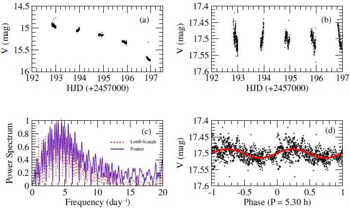
Fig. 1 (a) V band light curve during an outburst decline. Night to night the development of super humps was not observed. (b) V band light curve shifted to a quiescent magnitude, V = 17.5. (c) Normalized power spectrum showing both Lomb-Scargle Periodogram (red dotted line) and DFT power spectrum (violet solid line) for all data points. (d) Folded light curve with P1. The color figure can be viewed online.
The power spectrum obtained in two different ways is too noisy to reveal a true photometric orbital period. In Panel (c) of Figure 1 we show both the normalized DFT power spectrum and the LombScargle periodogram. The highest peak corresponds to a period P1 = 5.30 h; the folded light curve is contaminated by extra modulations but it still shows a sinusoidal behavior, so it is not clear if this is the orbital period of the system because the power spectrum contains several frequencies of similar amplitude.
3.2. Spectroscopic Results
The averaged spectrum for V767 Cyg is presented in Figure 2. The upper panel corresponds to the 2015 observations and the lower panel shows the 2016 run. The features are consistent with a typical dwarf nova during outburst. In both cases the continuum can be well approximated by a function Fλ ∝ λ−α, with α = 2.5. This spectral energy distribution is quite similar to that expected for an infinitely large steady state disc, i.e. Fλ∝ λ −7/3 (Lynden-Bell 1969).

Fig. 2 Averaged spectra of V767 Cyg for the 2015 and 2016 observational campaign showing the outburst state. The upper spectrum was obtained one day after our photometric observations, while the system was still in outburst decline. The bottom spectrum was obtained near maximum light, shown by the almost absence of Balmer emission lines.
3.3. Radial Velocity and the Orbital Period
Our 2015 spectroscopic observations were performed one day after our photometry, so the system was closer to its quiescent state. As we can see from Figure 2, during the 2016 spectroscopic campaing, the object was near its maximum light emission: the averaged spectrum shows an almost absence of emission lines.
Continuing with our purpose, we measured the Doppler shifts in the Hα emission line and in the center of the Hβ line, for those spectra obtained during 2015, as well as in the Hβ, Hγ, Hδ and Hϵ absorption lines, for spectra obtained in 2016, to generate RV curves. During the spectroscopic observational campaigns, the object was in an eruptive state.
Due to spectrograph flexions, the spectral line positions presented a small displacement that was corrected by monitoring the night sky line λ5577.338. After wavelength corrections were done, we carried out Doppler shift measurements. We measured the position of the lines in each spectrum, using the splot task from IRAF. We applied a single Gaussian curve to fit the line profiles.
We present the RV curve for Hα (2015 observational campaign) with its power spectra (normalized to compare DFT with a Lomb-Scargle periodogram) in Figure 3. The power spectra are less noisy than the photometric ones. The frequency of maximum amplitude corresponds to a period of P2 = 3.39 h.

Fig. 3 (a) Normalized power spectrum for the RV curve showing a DFT and Lomb-Scargle periodogram; both contain the P1 peak. (b) Folded RV curve with the frequency of maximum amplitude, fHα = 7.071 d−1. The color figure can be viewed online.
However, both power spectra also show several possible frequencies with similar amplitude. For the 3.39 h frequency, the RV curve is well fitted by a sinusoidal function. In this sense, the orbital period is more likely to be close to 3.4h instead of 5.30 h, in congruence with the U Gem class of CVs. We obtained the same frequency by analyzing, in the same way, the RV curve for the center of the H β line.
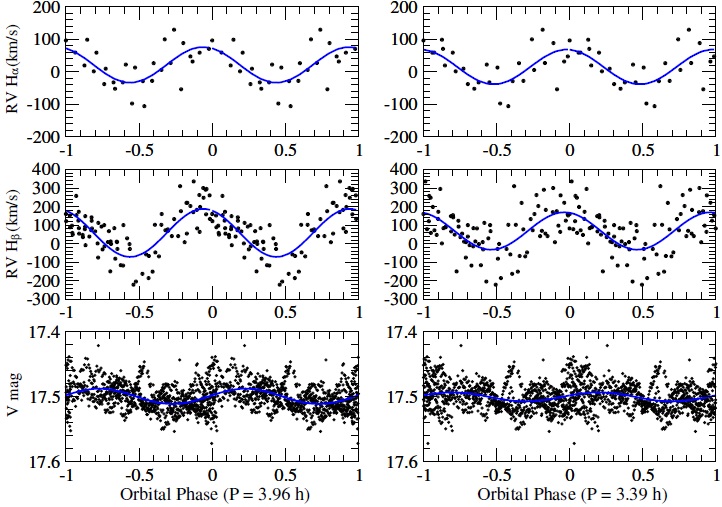
We repeat the same RV curve treatment and analysis for the Hβ, Hγ, Hδ and Hϵ absorption lines using the spectra obtained during the 2016 campaign. The results obtained for the Hβ RV curve are shown in Figure 4. In this case, the frequency of maximum amplitude corresponds to a period of P3 = 3.96 h, but again, the power spectra show other frequencies of similar amplitude; especially present are the photometric and the Hα frequencies.

Fig. 4 (a) Normalized power spectrum for the RV curve showing a DFT and Lomb-Scargle periodogram; both periodograms contain the P1 and P2 peaks. (b) Folded RV curve with the frequency of maximum amplitude, fHβ = 6.058 d-1, is well fitted by a sinusoidal function. The color figure can be viewed online.
Although we just show the Hβ RV curve, the results obtained by averaging other Balmer lines do not much improve our orbital period estimation for this observational campaign.
We carried out a non linear least-square fit to both spectroscopic data sets in the form of RV(t)= γ + K × sin(2πt/P + ϕ), where γ is the systemic velocity, K is the semi-amplitude of RV, and ϕ is the zero-phase. The resulting values of γ, K and are presented in Table 3.
Table 3 Radial velocity parameters.
| Line ID | γ (km/s) | K (km/s) | Phase shift ϕ |
|---|---|---|---|
| H α | 16.6 | 53.6 | 1.4 |
| H β | 58.4 | 129.2 | 0.79 |
In Figure 5 we present the three normalized power spectra mentioned above (V -band photometry, Hα and Hβ RV curves); we have marked P1, P2, and P3. In order to discriminate between the frequencies and derive the true orbital period, we applied the method described in Mennickent & Tappert (2001) and in Mennickent et al. (2002). As they explain, we fitted both spectroscopic data sets with a sine function corresponding to each maximum frequency and we measured the standard deviation (σ) for each fit. From there we generated 1000 artificial data sets with the same dispersion and time distribution as the originals data sets. We applied a Monte Carlo simulation, adding a random value from an interval ± 3σ to each data point of the fit function. Then we measured the highest frequency for each artificial data set, obtained after applying a Lomb-Scargle algorithm. The histograms for these values are shown in Figure 6. The peak at 6.058 d−1 (vertical blue dotted line) shows the highest peak for both RV curves, so the period favored with this methodology is P3 =3.96 h.


Fig. 6 Histogram of the maximum-peak frequency. Top, Monte Carlo simulation results for the Hα RV curve. Bottom, Monte Carlo simulation results for the Hβ RV curve. The color figure can be viewed online.
This result is congruent with the inset of Figure 5, where we show both spectroscopic periods, indicated with vertical dashed lines. The amplitude observed in the power spectrum for the photometric data set (green solid line) is higher for the P3 than for the P2 frequency, that gave us an idea for the true orbital period for V767 Cyg.
From the above, we ruled out P1 as the orbital period for V767 Cyg. In order to ensure that P3 is the orbital period, we folded the V-light curve and both RV curves with P2 and P3 as shown in Figure 7. The data show less dispersion and more coherence to the fit that corresponds to P3 = 3.96 h. So we conclude that P3 = 3.96 ± 0.29 h is the orbital period for V767 Cyg. The error corresponds to the FWHM of the maximum frequency for the Hβ line power spectrum.
4. DISCUSSION
According to the magnitude reported in the vsnet-alert 18748, during the 2015 event the system increased its brightens nearly 3 magnitudes, thus the system developed a normal outburst. This fact supports, in a good manner, our orbital period estimation because CVs with periods close to ≈ 4 h or longer do not exhibit superhumps. Such modulations are absent in the light curve. An advantage of the presence of superhumps in the light curve is the period excess relationship, which gives the mass ratio and other physical properties for the system.
However, according to Knigge et al. (2011), it is possible to obtain different physical properties from the orbital period of the CV. They updated the physical properties of the CVs by using systems that are transiting and therefore their masses and semi-major axes are very well determined. From there, they obtained semi-empirical relations to find masses, radii, temperatures, and spectral types of both the white dwarf and the main-sequence star companion. We used the data from their tables 6 and 8 to obtain the best physical parameters for V767 Cyg. Since those tables show only a portion of the full tables we used the full tables available online and we interpolated in order to find the best possibles values. These values are shown in Table 4, where the first row corresponds to the estimated value; the second and third rows are the errors for each physical parameter.
Table 4 Component parameters.
| Period | M2 | R2 | Teff2 | Spectral | M1 | R1 | Teff1 |
|---|---|---|---|---|---|---|---|
| h | M⨀ | R⨀ | K | Type (2) | M⨀ | 108 cm | K |
| 3.96 | 0.32 | 0.40 | 3 451 | M3.4 | 0.75 | 7.85 | 24 815 |
| +0.29 | +0.13 | +0.08 | +70 | +M3.0 | +0.16 | +1.10 | +2378 |
| -0.29 | -0.13 | -0.07 | -55 | -M3.7 | -0.16 | -0.07 | -2591 |
We obtained a mass ratio (q = M2 /
M1) of 0.43 for the estimated orbital period, which
is consistent with the previous classification of V767 Cyg as a SS Cyg dwarf nova,
so V767 Cyg was not mis-classified. The secondary mean density from Table 4 is
The mean density of the secondary star is a parameter that can be estimated from the system’s mass ratio (q) and the orbital period (P), by assuming that the star is filling its Roche Lobe, with a reasonable error of ≈ 5%. According to Eggleton (1983), if a star fills its Roche lobe, its mean density is given by
thus, the secondary star in V767 Cyg has a mean density of 7.1 g cm−3. This is in agreement with the value calculated from the best physical parameters listed in Table 4.
4.1. Uncertainty Propagation Estimation
Masses of WD in CVs range typically from 0.5 to 1.1 M⨀. In the absence of any plausible estimation for M1, a representative WD mass in a typical CV is the mean value M1 = 0.75 M⨀. In the case of M1, the uncertainty was taken from Patterson et al. (2005) (they used eclipsing binaries for their estimations). The statistical error of their calculations comes from the RMS of the mass distribution of WDs in their CVs sample, estimated as 0.16 M⨀. Also, Patterson et al. (2005) proposed a mass-radius relation for the secondaries where the estimated uncertainty for M2 and R2 is 25% and 8%, respectively.
Additionally to these uncertainties, we calculated the uncertainty for M2 and R2 that arises from the uncertainty of the orbital period observed. To do this, we interpolated the track models presented in Knigge et al. (2011). To calculate the uncertainty that appears in Table 4 we added both uncertainties, the one from the M1 = 0.75 M⨀ assumption and the one from the error in the orbital period.
For the rest of the parameters (Teff2, spectral type of M2, R1 and Teff1) we only propagated the uncertainty in the orbital period (3.96 ± 0.29h) using the track models from Knigge et al. (2011) to calculate the corresponding upper and lower value that appears in Table 4.
5. CONCLUSION
For the binary V767 Cyg, classified as an SS Cyg system in the Downes catalogue, there were no previous data in the literature reporting the value of its orbital period. Taking this evidence as a starting point, we conducted observations in order to contribute to this measurement. We performed during 2015 and 2016, photometric and spectroscopic observations to constrain the value of its orbital period. In 2015, during the photometric run, the object was found to be in an eruptive state, which did not allow us to reliably determine the orbital period from the analysis of the light curve due to its complexity. The period we obtained from the light curve was 5.3 h. However, with spectroscopic observations obtained in the same observational campaign, we measured the Doppler shift in the emission line Hα, because the system was close to its quiescence state. The emission lines are produced in the optically thin accretion disk and reflect closely the orbital motion of the binary system. Analyzing the RV curve for the emission line we estimated a period of 3.39 h.
During the 2016 campaign, the system was again caught in the eruptive state, as suggested by the almost absence of emission lines; the object was close to its maximum brightness. We analyzed the RV curve with the absorption line Hβ and we found a period of 3.96 h, slightly larger than that determined for the Hα line. To discriminate between the possible frequencies and to determine the true orbital period we carried out a Monte Carlo simulation and a non-linear least squares fit to the three data sets to obtain the best coherence and lowest dispersion. We found that the photometric and spectroscopic data were best fitted with the period of 3.96±0.29 h. The error corresponds to the FWHM of the maximum frequency of its power spectrum.
This article is based upon observations acquired at the Observatorio Astronómico Nacional in the Sierra San Pedro Mártir (OAN-SPM), Baja California, México.

