


 text new page (beta)
 English (pdf)
 Article in xml format
 Article references
 Send this article by e-mail
 Cited by SciELO
  Similars in
SciELO
Similars in
SciELO 
 Permalink
1. INTRODUCTION
Massive stars (≳ 25 M⊙) inject during their lives mechanical energy into the interstellar medium through their stellar winds (with a wind terminal velocity υw =2000 km s−1 and mass loss rate of ˙M ≈ 10−6 to 10−5 M ⊙ yr−1; (e.g. Friend & Abbott 1986). The stellar winds could sweep up the interstellar medium creating a dense shell filled with very hot gas known as wind bubble with a size of a few 10 pc and superbubbles with sizes ≈ 100 pc (in the case of a shell created by stellar winds of star associations). During the evolution of this bubble, the transfer of energy into the interstellar medium (ISM) can be carried out by radiative luminosity (L∗) and by mechanical luminosity due to winds (Lw = Mυ2w).
The wind bubble formation begins when the massive star first forms an H II region with size of about 1 pc in a very high density medium. During the star’s main sequence and WR phases, the expansion of the ionized gas is driven by the hot shock stellar wind bubble.
In general HII regions have spherical geometry in a homogeneous density medium. Nevertheless, some present an asymmetric geometry when they are in an inhomogeneous medium. These asymmetries can be classified according to their morphology: (I) bow shocks of an ionizing star moving supersonically through a molecular cloud (Van Buren et al. 1990; MacLow et al. 1991). (II) “Champagne flow” where it is assumed that the massive star is born in a medium with density gradients (Tenorio-Tagle 1979). (III) bipolar morphology resulting from the confinement of the ionized gas by a flattened structure of neutral gas and dust (Campbell 1984; Rodriguez et al. 1988).
A bubble created by a massive star can be explained as a classical HII region. One scenario indicates that the creation of bubbles is driven by the pressure difference between the ambient ISM and the ionized gas of the HII region. The analytical approximation to the expansion of an HII region in a homogeneous ambient medium does not consider the stellar winds (Spitzer 1978). A second scenario is the H II region expansion in the presence of a stellar wind in a uniform medium (Dyson & Williams 1980). An example of the first case was presented by Martins et al. (2010). They found that for the bubble RCW 79, the mechanical wind luminosity is about 10−3 the ionizing luminosity in the RCW79 nebula indicating that the formation of the ring nebula could be attributed to the radiation pressure of the star. The importance of stellar winds of massive stars for the formation of bubbles and superbubbles is still discussed.
On the other hand, the standard model of Weaver et al. (1977) and Chu & Mac Low (1990) describes these bubbles as extended bubble structures of shock-heated gas emitting X-rays, surrounded by a shell of swept-up and cool ISM observed as optical emission. This model considers two shocks: a principal shock of swept-up ISM compressed to a thin shell at a temperature of about 104 K and a secondary shock of heated gas at temperatures 106 − 107 K.
Considering this last scenario, a ring nebula is expected around massive stars. However, the optical survey of Wolf-Rayet ring nebulae (Heckathorn et al. 1982; Chu et al. 1983; Miller & Chu 1993; Marston et al. 1994) shows that only about a fourth of the ≈ 150 observed Galactic Wolf-Rayet stars are associated with ring-like nebulae (Wrigge et al. 2005). Also, in a recent work, Chu (2008) and Chu (2016) analyzed HST observations of the H II region N11B (around the OB association LH10). The HST images of this HII region do not show ring-like morphological features. However, the long slit spectrogram of the [N II] λ6583 line shows splitting, indicating the existence of an expanding shell of ≈ 15 pc with Vexp of 15-20 km s−1. The conclusion of Chu (2016) is that the expansion velocity is associated with weak shocks within the photoionized medium. This medium does not produce a large enough density jump to form a bright shell. If the medium is neutral, then there is a density contrast due to the strong shock, and it is easier to observe a ring nebula in HI emission than in the optical range.
Regarding the X-ray emission of superbubbles, it is important take into account that the original work of Weaver et al. (1977) overestimated the observed X-ray luminosity in some bubbles. And for example, others studies like Harper-Clark & Murray (2009) and Rogers & Pittard (2014) underestimate the X-ray emission (see Castellanos-Ramírez et al. (2015) for more information). Therefore, from a theoretical point of view, the X-ray luminosity in a bubble is expected. And, there seems to exist a correlation between the kinematics of the bubble and the X-ray and optical emission.
The study of the kinematics and X-ray emission of the superbubbles presented by Oey (1996) proposed two superbubble categories in terms of dynamical data: high-velocity superbubbles and lowvelocity superbubbles, the latter type being more consistent with the standard model. For the high velocity type an additional source of energy as a supernova explosion was proposed (Rodríguez-González et al. 2011).
Also, X-rays observations of the superbubbles N70 and N185 located in the Large Magallanic Cloud ( an ideal laboratory to observe objects in X-rays due to their low extinction), show X-ray emission inside the optical shell (Reyes-Iturbide et al. 2014; Zhang et al. 2014) and present an excess of X-ray emission. Therefore, to explain the shell formation and the excess of X-ray emission Rodríguez-González et al. (2011) and Reyes-Iturbide et al. (2014) included an additional source of energy.
On the other hand, there are some bubbles that has been observed in optical and X-ray emission; e.g. NGC 6888 (Gruendl et al. 2000; Moore et al. 2000; Toalá et al. 2016); S308 (Toalá et al. 2012); NGC2359 (Toalá et al. 2015); NGC3199 (Toalá et al. 2017).
In this work we address the problem of the correlation between kinematics and X-rays emission in the bubble RCW120 by using observations in the optical from the Fabry-Perot interferometer PUMA and X-ray data from CHANDRA, with the help of hydrodynamic numerical simulations.
1.1. RCW120
RCW120 is a Galactic bubble located at 1.3 kpc from the Sun (Zavagno et al. 2007) bounded by a massive, dense shell with mass Msh ≈ 1200 − 2100 M⊙ (Deharveng et al. 2009). It is also called Sh 2-3 or Gum 58 and has a diameter of 1.9 pc (Anderson et al. 2015). The ionizing star of RCW120, CD-38◦11636 or LSS 3959 is an O8 type star (Georgelin & Georgelin 1970; Avedisova & Kondratenko 1984; Russeil 2003; Zavagno et al. 2007) located at αJ200 =17h 12m 20.6s, δJ200 =-38°29’26”. Its magnitude is B = 11.93 and V = 10.79 (Avedisova & Kondratenko 1984), with M∗ ≈ 30 M⊙. K-band images of the ionizing star of RCW 120 from 2MASS and SINFONI suggest that the star is double, with a companion of the same type (Martins et al. 2010). Table 1 summarizes the characteristics and properties of RCW 120.
Table 1 Characteristic of rcw 120 and its ionizing star.
| Bubble Parameters | Value | Reference |
|---|---|---|
| Names | Sh2-3 | Sharpless (1959) |
| Distance [kpc] | 1.34 | Zavagno et al. (2007) |
| Radius [pc] | 1.9 | Anderson et al (2015) |
| no [cm-3] | 2000-6000 | Anderson et al. (2015)) |
| n(H2) [cm-2] | 1.4×10²² | Torii et al (2015) |
| n(H2)ring [cm-2] | 3.22×10²² | Torii et al. (2015) |
| Mring [M⊙] | 3100 | Torii et al. (2015) |
| 2000 | Deharveng et al. (2009) | |
| M(HII) [M ⊙] | 54 | Zavagno et al. (2007) |
| rring [pc] | 1.7 | Torii et al. (2015) |
| t[Myr] | 0.4 | Torii et al. (2015) |
| Zavagno et al. (2007) | ||
| Ionizing star Parameters | ||
| Age [Myr] | 5 | Martins et al. (2010) |
| B [mag] | 11.93 | Avedisova & Kondratenko (1984) |
| V [mag] | 10.79 | Avedisova & Kondratenko (1984) |
| J [mag] | 8.01 | Avedisova & Kondratenko (1984) |
| H [mag] | 7.78 | Martins et al. (2010) |
| K [mag] | 7.52 | Martins et al. (2010) |
| M∗ [M⊙] | 30 | Martins et al. (2010) |
| log (L∗/[L⊙] | 5.07 | Martins et al. (2010) |
| teff [K] | 37500 | Martins et al. (2010) |
| ˙M [M ⊙ yr-1] | 1.55×10⁻⁷ | Martins et al. (2010) |
| Martins et al. (2010) | ||
| L0 [erg s-1]a | 1038 | Martins et al. (2010) |
aL0 is the ionizing photon luminosity.
Current studies carried out with the NANTEN2, Mopra, and ASTE telescopes reveal two molecular clouds associated with RCW 120, with a velocity separation of 20 km s-1 (Torii et al. 2015). The cloud at -28 km s-1 is located just outside the opening ring while the cloud at -8 km s-1 traces the infrared ring (Anderson et al. 2015). Hα Fabry-Perot observations of RCW 120 have been reported in the survey CIGALE of the Milky Way and the Magellanic Clouds (Le Coarer et al. 1993); they were obtained with a 36-cm telescope (La Silla, ESO) by Zavagno et al. (2007). These authors found LSR radial velocity of ionized gas ranges of −8 to −15 km s−1 and they did not find evidence for expansion of the ionized hydrogen associated with RCW 120.
RCW120 is possibly a triggered star formation region (like RCW 82, RCW 79), embedded in a molecular cloud (Zavagno et al. 2007). 2MASS, Spitzer and Herschel observations of this bubble reveal the existence of young stellar objects located in the massive condensation in the surrounding bubble (Deharveng et al. 2009; Zavagno et al. 2010) indicating active star formation in this region. Since there should be shock compression triggering the star formation, we obtained Fabry-Perot data at [SII]λλ6717,6731 Å because it is easier to identify shocks in [SII] rather than in Hα; this is because of the higher [SII]/Hα line-ratio and also because [SII] velocity profiles of each component are narrower than Hα velocity profiles due to the larger atomic weight of [SII].
The layout of the paper is as follows. The observations and data reductions using the Fabry-Perot interferometer are presented in § 2. In § 3 we present the analysis of the kinematics of RCW 120 as well as its morphology and spatial density distribution. In § 4 we show the numerical evolution of the X-ray emission and shell dynamics of a bubble with the physical characteristics of RCW 120. The discussion and conclusions are presented in § 5.
2. OPTICAL OBSERVATIONS AND DATA REDUCTIONS
The observations were carried out in July 2014 using the 2.1 m telescope of the Observatorio Astronómico Nacional of the Universidad Nacional Autónoma de México (OAN, UNAM), at San Pedro Mártir, B. C., México. We used the UNAM scanning Fabry-Perot interferometer PUMA (Rosado et al. 1995). We used a 2048×2048 Marconi2 CCD detector with a binning factor of 4 resulting in a FoV of 10′ and dimensions of 512 × 512 pixels with a spatial sampling of 1′′.3 pixel−1.
We obtained [SII]λλ6717,6731 Å Fabry-Perot data cubes of RCW120. The Fabry-Perot interferometer has a finesse of ≈ 24 leading to a sampling spectral resolution of 0.41 Å (equivalent to a sampling velocity resolution of 19.0 km s−1 at 6717 Å) and a free spectral range of 20Å (equivalent to a velocity range of 929 km s−1 at 6717 Å). The spectral resolution was achieved by scanning the interferometer free spectral range through 48 different channels producing velocity cubes of 512 × 512 × 48 (Rosado et al. 1995). The interference filter used was centered on 6721 Å) with a bandpass of 20 Å. To calibrate the [SII] cube we used a neon lamp (6717.04 Å wavelength calibration) and the calibration data cube had dimensions of 512 × 512 × 48. We also obtained a set of direct images in Hα and [SII] using PUMA in its direct imaging mode (see Figure 1). The exposure time of each of the direct images was 120 s. Observational and instrumental parameters are listed in Table 2.
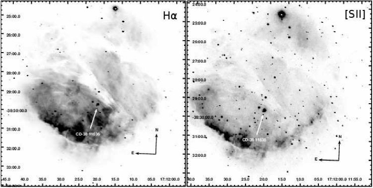
Fig. 1 Direct images of RCW120. The left panel shows the Hα emission and the right panel shows the [SII]λλ6717,6731Å emission. A white arrow shows the ionizing star position (Sh2-3).
Table 2 Observational and instrumental parameters.
| Parameter | Value |
|---|---|
| Telescope | 2.1m (OAN, SPM) |
| Instrument | PUMA |
| Detector | Marconi CCD |
| Scale plate | 0’’.33/pix |
| Binning | 4 |
| Detector size | 2048 × 2048 [pixels] |
| Central Lambda | 6720 [Å] |
| Banswidth | 20 [Å] |
| Interference Order | 322 at 6717 [Å] |
| Free spectral range | 929 [km s-1] |
| Exposure time calibration cube | 0.5 s/channel |
| Exposure time object cube | 120 s/channel |
The images were reduced using standard IRAF1routines. The data reduction and analysis of the Fabry-Perot data cubes were performed using the CIGALE software. CIGALE allows flat field correction, wavelength calibration, construction of velocity maps and derivation of radial velocities, identification of sky-lines, profile extraction and fitting. In this case, the data cubes in the [SII] lines are not contaminated by sky line emission. In the spectral window, the data cubes do not show any sky lines. No spatial or spectral smoothing was applied to the data. The CIGALE data reduction process allows to compute the parabolic phase map from the calibration cube. This map provides the reference wavelength for the line profile observed inside each pixel. Also, we can compute from the phase map the wavelength, monochromatic, continuum maps.
The extraction of the kinematic information from the Fabry-Perot data cube was done using the radial velocity map of RCW120. This map was obtained using the barycenter of the [SII]λ6717 Å (used as the rest λ) velocity profile at each pixel. The radial velocity profiles were fitted by the minimum number of Gaussian functions after deconvolution by the instrumental function (an Airy function). The result of this convolution is visually matched to the observed profile. The computed width of the Gaussian functions is taken as the velocity dispersion (of the velocity component corrected by the instrumental function with a width of 38 km s−1).
3. DATA ANALYSIS
Figure 1 shows the direct images of Hα and [SII]λλ6717,6731 Å emission-lines obtained with PUMA. The ionizing star is marked with a white arrow. We can see a well defined ionization front (IF) of RCW120 located in the southern region of the nebula showing a section of shell formed of dense material (shocked gas emitting in [SII] emission lines). This region corresponds to the dust condensations #1 and #7 (see Deharveng et al. 2009) where more young stellar objects (YSO) are located. On the opposite side of the IF an open structure is observed.
3.1. Kinematics of the Nebula
Our Fabry-Perot data allow us to identify the global trends of the kinematics of RCW120 in [SII] emission. With the Fabry-Perot interferometer PUMA it is possible to study both the large scale motions and the punctual motions, like expansion velocities, unlike classical long-slit spectrometers which are limited by the aperture spectrometry and give information of a small part of the object.
Figure 2 shows a mosaic obtained with the observed fields with the [SII] radial velocity profiles integrated over windows of 20×20 pixels size (26”×26”) overlaid on a [SII] image. The x and y axis indicate the (x,y) position of each integrated velocity profile. In this figure we can see that the brightest emission is coming from the southern region of nebula; the two [SII]λλ6717,6731Å lines are detected and are separated by about 15 channels (equivalent to 285 km s−1). Profiles from the northern region show different intensities between the two [SII] lines, whereas the profiles from the southern region seem to have the same intensity. Since both lines λ6717Å and λ6731Å are emitted by the same gas, we will focus on the brighter line ([SII]λ6717Å).
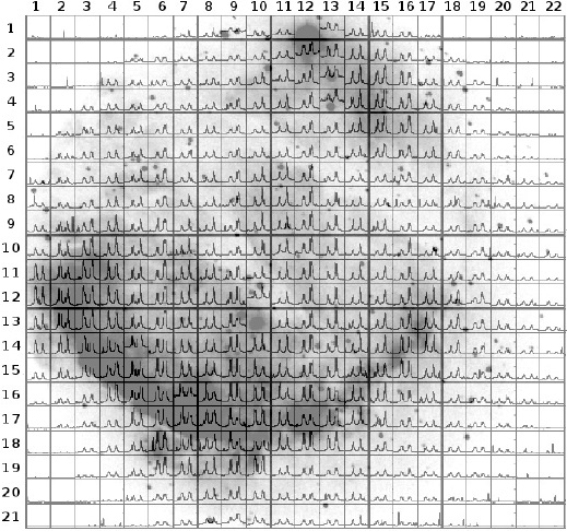
Fig. 2 Some examples of the [SII] radial velocity profiles (20×20 pixels velocity profile plots) of the different regions of RCW 120 superimposed on a [SII] emission velocity map at −21 km s−1 (gray color). The numbers at top and left indicate the coordinates of the position of the profiles.
We have fitted the velocity profiles shown in Figure 2 using Gaussian functions, considering those with a significant signal to noise ratio and taking into account the brighter line ([SII]λ6717Å). We corrected the observed FWHM to account for effects that broaden the lines. The instrumental broadening σinst was done by the deconvolution of the Airy function, and in this case corresponds to 38 km s−1. We computed the thermal broadening according to σth√82.5(T4/A) where T4 = T /104 K and A is the atomic weight of the atom. The correction for thermal broadening to the [SII] is about 1.6 km s−1 (Asulfur =32.065u). Compared with the instrumental broadening this has no effect upon our results. The fine structure broadening correction σth is important for hydrogen and helium recombinations lines, but not for metal lines such as [SII] and [NII] (García-Díaz et al. 2008), so this correction is not required. The turbulence broadening σtr is related to other motions, like nonthermal motions. It is often complicated by superpositions along the line of sight of emission completely independent of the observed structure (Courtés 1989); therefore the turbulence broadening has no effect upon our conclusions.
From the velocity profile fit we found that the profiles in the northeastern region of the nebula (on the side of the open structure) are complex and broad, indicating the presence of different motions in that region. The profiles in the southern region of the bubble present single broad [SII] profiles corresponding to the radial velocity of the nebula. In the spectral window, the data cubes do not show any sky lines. No spatial or spectral smoothing was applied to the data.
In Figure 3 we present the spatial distribution of velocity profiles with single component (dark gray) and with double velocity components (light gray). As can be seen in this figure, most of the regions with two velocity component are located in the northeast side of the nebula (the region of the open structure) and some are in the west side of the nebula.
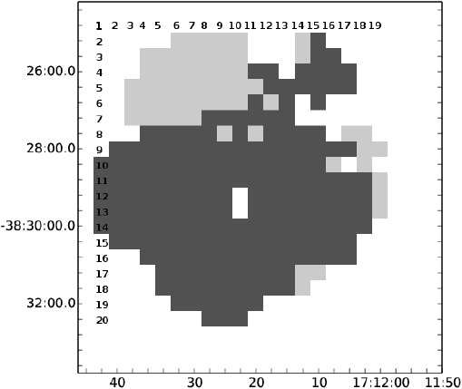
Fig. 3 Spatial distribution of velocity profiles with single and double components. Each region represents the same as in Figure 2 with a size of 20×20 pixels. Profiles with single component are shown in dark gray and profiles with double velocity components in light gray.
In order to show the differences between bright components we show in Figure 4 the radial velocity profiles of one region with a single velocity component and another with two velocity components. The x-axis in the profiles is given in channels (each channel has associated a wavelength) and the y-axis gives the intensity of the line in arbitrary units. The single component of the velocity profiles corresponds to the radial velocity of the nebula. Velocity profiles with two components are called extreme velocity components. We shall refer to these as Vmain (representing the radial velocity of the nebula) and Vsec (associated with other movements). These are marked as No. 0 and No. 1, respectively.
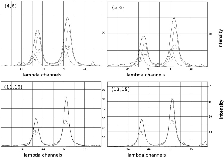
Fig. 4 [SII] radial profiles of four regions obtained with Fabry-Perot. At top left the (x,y) position of the extracted integrated velocity profile according to Figure 2 is shown. Top profiles are composite, bottom profiles are single. The profiles were integrated over boxes with a 20×20 pixel size. Th x-axis in the profiles is given in lambda channels and the y-axis is the intensity in arbitrary units. Both [SII] lines at 6717 Å and 6731 Å are detected. Decomposition of each profile is indicated by thin lines. The resulting profiles are shown as hollow circles with numbers. The dotted line represents the sum of all fiftted components.
Figure 5 displays the velocity maps of the components obtained from the fit profiles. The top panel shows the velocity map of the Vmain component. The bottom panel shows the velocity map of the Vsec component. The highest LSR velocity values originate in the southeast side of the nebula. The VLSR presents a gradient of about ∆VLSR =60 km s−1 (varying between −74 km s−1 and −6 km s−1). This velocity gradient matches the CO distribution of the red cloud towards this nebula presented by Torii et al. (2015).
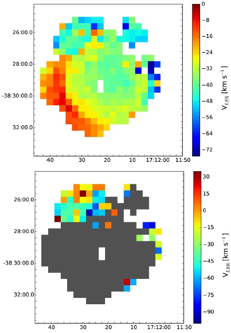
Fig. 5 Velocity maps of the components obtained from the fitted profiles. Top panel: velocity map of the Vmain component. Bottom panel: velocity map of the Vsec component. The regions with a single velocity component are shown in gray. The color figure can be viewed online.
The expansion velocity determined for the regions with composite profiles is Vexp =20 km s−1. This value was calculated using the expression: Vexp = (Vmain− Vsec)/2.
3.2. Emission-line Ratio Maps and Electron Density
Figure 6 shows the [SII]/Hα line-ratio map. We can see that the highest values are located in the IF and in the northern region of the nebula, showing the shocked gas in this region. In the west region of the nebula the [SII]/Hα values span from 0.2 to 0.3, while in the east region the values span from 0.1 to 0.2. These differences indicate that the ISM is not homogeneous. In Figure 6 we can see that the highest [SII]/Hα line-ratio values correspond to the northern region of the nebula where the profiles with largest velocity values are located.
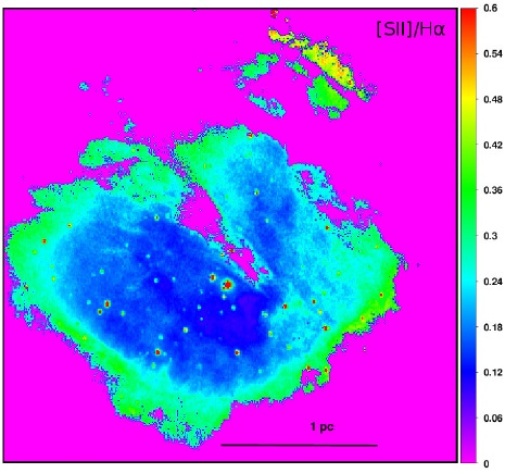
Fig. 6 [SII]/Hα line-ratio map. North is up and east is to the left. The color figure can be viewed online.
From our [SII] data cube, where both 6717Å and 6731Å lines are detected, we were able to compute [SII]λ6717/[SII]λ6731 line-ratios (see Figure 7). The line-ratio values span from 0.3 to 1.5. The lowest [SII]λ6717/[SII]λ6731 line-ratio values are located inside on the nebula.
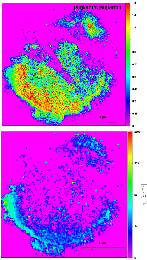
Fig. 7 Top panel: I([SII] λ6717)/I([SII] λ6731) ratio. Bottom panel: Electron density map in units of particles per cm3. North is up and east is to the left. The color figure can be viewed online.
In order to explore the morphology of the nebula RCW 120, we obtained the electron density map, assuming a constant electron temperature of 10000 K, corresponding to the expected conditions in H II regions, and using the [SII]λ6717/[SII]λ6731 line-ratio map.
The electron density map was computed using
where x is defined as x ≡ 10−4 ne T1/2 and T is the electron temperature in units of 104 K (McCall et al. 1985).
In both cases we do not correct for differential extinction between Hα and [SII] and the two lines of [SII]λλ6717,6731 because these lines are too close rendering the correction insignificant.
In the lower panel of Figure 7 we present the electron density map. We obtained a maximum density of ≈ 3000 cm−3 in the southern region of RCW 120, and we fixed a minimum density of 0.03 cm−3 (in order to run numerical models). Also, from this figure we can see that the spatial variation of electron density, ne, in the southern region of the nebula presents a high density (≈ 3000 cm−3), and it is possible to appreciate two arch-like structures (south-southwest and south-south-east). The external one shows electron density values between 3 and 400 cm−3; while the internal arch has values between 3 and 40 cm−3. The presence of two arch-like regions could be due to the difference in density of the clouds towards which the H II region seems to be evolving, as proposed by Torii et al. (2015). The lower electron density values are found in the northern region of the nebula; these differences in density cause a faster expanding material in this region allowing the ionized gas to possibly break the shell. This is known as the “champagne phase” (Tenorio-Tagle 1979).
4. CHANDRA X-RAY OBSERVATIONS AND GAS DYNAMIC SIMULATION OF RCW 120
RCW120 has been observed with the Chandra X-Ray Observatory using the Advanced CCD Imaging Spectrometer (ACIS) ObsID 13276 and 13621, with a exposure time of ≈30 ks and ≈49 ks, respectively. From these observations, Townsley et al. (2018) found extensive diffuse X-ray emission coming from RCW 120 tracing hot plasma through a breach in the northeast side of the bubble and out into the surrounding ISM.
Several point sources have been identified, 678 X-ray point sources have been detected in the catalog for RCW 120 produced by Getman et al. (2017) as part of the SFiNCs project. Some properties of stellar clusters in the SFiNCs regions, including RCW 120, are presented in: Getman et al. (2018) and Richert et al. (2018). On the other hand, Townsley et al. (2018) produce an extended Chandra X-ray source catalog of point 999 X-ray sources in RCW 120, including even fainter X-ray sources found by Getman et al. (2017).
In order to explore the X-ray emission and the shell dynamics of the RCW120, we performed 3D numerical gas dynamics simulations. In this case we did not include photoionization nor radiation pressure because although massive stars form around an HII region before its powerful wind interacts with the surrounding medium (ionized gas), it is not entirely clear when one effect dominates over the other. As we mention above, in some cases, the creation of bubbles is simply driven by the pressure difference between the ambient ISM and the ionized gas of the H II region, and the effect of mechanical energy due to stellar wind is negligible.
Also, Mackey et al. (2016) compared synthetic infrared intensity maps made by numerical simulations with some Herschel infrared observations for RCW 120. They concluded that, in order to obtain the shape and size of a bright arc in the infrared waveband, they had to include stellar winds in their simulations.
On the other hand, Martins et al. (2010) point out that the dust emission at 24 μm (the same wavelength used by Mackey et al. 2016) does not favor a strong influence of stellar winds.
Recently, Gvaramadze et al. (2017) reported both observations and numerical simulations of an H II region IRAS 18153-1651. They found an optical arc near the center of the nebula, and suggested that this arc is the edge of a wind bubble together with the H II region produced by a B star. They validated their hypothesis with analytical calculations of both the radius of the bubble and that of the H II region which fitted the observations. Also, they obtained synthetic Hα and 24 μm dust from 2D numerical simulations of radiation hydrodynamics. Their results are in good agreement with the observations for the morphology and the surface brightness.
In order to support the use of only stellar wind in our simulations, we followed the work of Raga et al. (2012). They obtained an analytical model for an expanding H II region driven by stellar winds and ionizing radiation, both of them coming from the central source. The transition between the two phases is related to the λ parameter (see equation (29) in Raga et al. 2012. and equation (26) in Tinoco-Arenas et al. 2015):
Basically, they concluded that if λ > 1, then the expansion of the region is described by the model for a wind-driven shell with a negligibly thin H II region.
In such way, we calculated the λ-parameter in terms of the values used in our numerical simulations (see Table 3); we obtained λ > 1. Therefore, as a good approximation, we can consider only the effects of a stellar wind in order to study the X-ray emission in our numerical models.
Table 3 Initial conditions of the numerical simulations.
| Model | υterm [km s-1] | ˙M[M⊙ yr-1] | n0[cm-3] | T0 [K] | Log10 Lw |
|---|---|---|---|---|---|
| M1 | 2313 | 2.7 × 10⁻⁷ | 2000 | 100 | 5.4 L⊙ |
| M2 | 2313 | 2.7 × 10⁻⁷ | 3000 | 100 | 5.4 L⊙ |
| M3 | 2313 | 2.7 × 10⁻⁷ | 6000 | 100 | 5.4 L⊙ |
We perform a set of three different numerical simulations using the Walicxe-3D code (see Esquivel et al. 2010; Toledo-Roy et al. 2014). This code solves the hydrodynamic equations on a three dimensional Cartesian adaptive mesh using a second-order finite volume conservative Godunov upwind method, with HLLC fluxes (Toro et al. 1994) and a piecewise linear reconstruction of the variables at the cell interfaces with a Van Leer slope limiter. Additionally, the code includes an artificial viscosity to stabilize the simulation. The energy equation includes the cooling function appropriate to describe the cooling of the shocked wind material. The cooling function for different metallicities, was obtained from the freely available chianti database (Dere et al. 1997; Landi et al. 2006).
The computational domain was a cube of 5 pc side, with a uniform medium of number density n0 and temperature T0 (see below). We used 5-levels in the adaptive grid with a maximum resolution of 256 points along the x, y and z axes.
Our numerical models considered appropriate values of the stellar wind velocity and mass injection rate for one single O8V star (see Sternberg et al. 2003 & Mackey et al. 2015 for the mass used in the simulation). The star was placed at the center of the box simulation and its stellar wind was imposed over a region of 5 pixels, corresponding to a physical radius of 0.08 pc. In this region we impose a steady-state spherical stellar wind solution with a ∝R2w density profile, such that: ˙M=4πρV∞R-2w. Also, the energy injected by the stellar wind must satisfy E = ρ|u|2 /2 + P/(γ − 1), with P the pressure due to the wind. Moreover, in order to improve the steady-state wind, we included a slope in velocity such that υ∞∝R-1w.
We explored three values of n0, the cloud density; these were: 2000, 3000 and 6000 cm−3. Table 3 shows the initial physical properties for the three numerical models, M1, M2 and M3. Column 1 indicates the model. Column 2 shows the wind velocity. Column 3 shows the mass loss rate. Columns 4 and 5 show the density and temperature of the surrounding environment. Column 6 shows the luminosity. We used a super-solar metallicity for the wind and a sub-solar metallicity in the interstellar medium, 3 and 0.3 Z⊙, respectively (see Castellanos-Ramírez et al. 2015). We carried out time integrations from t = 0 up to t = 0.4 Myr for all the models.
4.1. Numerical Results
The evolutionary X-ray emission for the models was computed using emission coefficients in the low-density regime taken from the chianti data base as function of the metallicity (see Figure 2 in Castellanos-Ramírez et al. 2015) in the band 0.6 to 10 keV (soft and hard X-ray band). Figure 8 shows the temperature, column densities and intrinsic X-ray emission maps (upper, middle, and lower panels, respectively), for the models M1, M2 and M3 (left, center and right panels, respectively) at t = 400 kyr. From the column density maps, one can see the radius of the shell driven by the stellar wind. As we expect, the model M3, a denser interstellar medium, has a small shell radius. On the other hand, we cannot see a contribution to the Xray emission coming from the shocked environment (by the leading shock). In the case of RCW120 this shell is very dense and the expansion velocity is around 20-40 km s−1. In the post-shock region the gas has a temperature around tens of thousands K, i.e. it would show optical emission. Nevertheless, a weak X-ray emission region is predicted in the nonshocked wind region, the very low dense gas region (see also the upper panel in Figure 9).
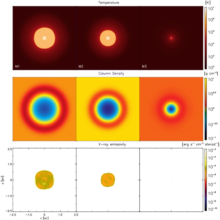
Fig. 8 Temperature, column density and intrinsic X-ray emission maps (upper, middle and lower panels, respectively) at an evolutionary time of 400 kyr. The results of models M1, M2 and M3 are presented. The color figure can be viewed online.
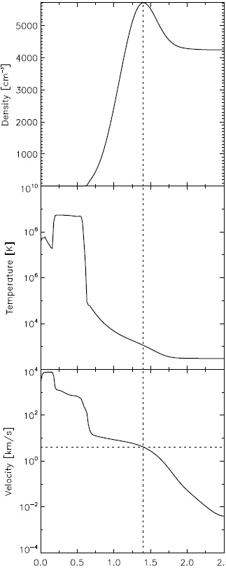
Fig. 9 Density, temperature, and velocity (upper, middle, and lower panels, respectively). As explained in the text, the regions of higher values for the density (marked with a dotted line) correspond to lower values to temperature and velocity and conversely. Moreover, the velocity value obtained in our numerical simulations (≈ 4 km s-1) is in agreement with the observational values.
In addition, the time when the models reach their maximum X-ray luminosity value is different for every model, as one would expect. It is about 60 kyr for model M1, 90 kyr for model M2 and 210 kyr for M3. Nevertheless, the intrinsic X-ray emission is about two orders of magnitude less than the X-ray emission from the central star of RCW120 (as we can see in the lower panels of Figure 8). In this way, the X-ray luminosity in this region has a value too low to be detected.
Therefore, from our numerical simulation we do not expect a detectable X-ray emission from the shocked gas of RCW120 although the temperature reaches 107 K. Table 4 shows the results for models M1, M2 and M3. Column 1 indicates the model. Columns 2 and 3 show the position and width of the optical shell (the shocked interstellar medium). Columns 4 shows the total soft X-ray luminosities at t = 400 kyr and Column 5 the maximum value of the soft X-ray luminosity reached by this numerical bubble in the band: 0.6 to 10 keV.
Table 4 Numerical results.
| Model | RShell [pc] | ∆RShell [pc] | Lx [x1029 erg s-1] | Lx,max [x1029erg s-1] |
|---|---|---|---|---|
| M1 | 2.40 | 0.72 | 1.32 | 4.48 |
| M2 | 2.12 | 0.68 | 1.61 | 4.88 |
| M3 | 1.52 | 0.53 | 2.66 | 5.22 |
Note that the external shell does not show X-ray emission despite the fact that the main source of Xray emission in bubbles is the medium swept up by the shock front. The shock wave rises the temperature of the gas and the maximum temperature (the post-shock temperature) is around 107 K for stellar wind velocities of ≈ 103 km s−1. In order to see this behavior more clearly, we present the density, temperature and velocity behavior as a function of the radius in Figure 9. We note, again, that the zone of very low density corresponds to high temperature as well as high velocity. When the density increases (upper panel in Figure 9), the other variables decrease (middle and lower panels in Figure 9). On the other hand, as shown in Figure 9 (bottom panel), the numerical value of the velocity obtained from the simulations, ≈ 4 km s−1 for RCW 120, is in good agreement with the expansion velocity from the observational data, which is in the range 20-40 km s−1 at a radius of 1.9 pc.
On the other hand, the density of the external shell is, at least, 4 times larger than the interstellar medium density, for an adiabatic expansion of a supersonic gas. However, in the case of a bubble evolving into dense ambients (i.e. the maternal cloud) its external shell loses an important fraction of its thermal energy because of radiative processes (cooling). The temperature of the gas of the outer shell drops from 107 K to 104 K in a cooling time given by,
where Eth is the thermal energy, Lrad is the cooling rate, k is the Boltzman constant, n is the numerical density, T the gas temperature, Z is the metallicity of the gas, and Λ(Z,T) is the cooling function as a function of Z and T. We can also re-write the cooling time (for a gas with initial temperature of 107 K) as
where the cooling function values were obtained from Castellanos-Ramírez et al. (2015). Using equation 4 we calculated the cooling time t = 1.25 × 10⁴, 8.34 × 10³, and 4.17 × 10³ yr, for the models M1, M2 and M3, respectively. Therefore, in the case of RCW120, we expect that the gas within the external shell remains at a temperature around tens of thousands K.
Therefore, in order to reproduce the shell size and width, our simulation predicted the average numerical density of the ambient medium (in southern region of the object) between 3000-5000 cm−3 and an interstellar medium density around 1000 cm−3 for the northern region of RCW 120.
5. DISCUSSION AND CONCLUSIONS
We analyzed the kinematics and the predicted X-ray luminosity of the galactic bubble RCW 120 using the PUMA Fabry-Perot interferometer and 3D numerical simulations. From the PUMA direct images we found that the Hα and [SII] emission (see Figure 1) show a diffuse “halo”, but the [SII] image shows the ionization front in the southern region of the nebula. In both cases the halo is not perfectly symmetric and is more extended toward the northern region of the nebula. We found that the higher [SII]/Hα ratios are located in the northern region of the nebula.
Kinematic information of RCW120 in [SII] line emission obtained here revealed that the LSR radial velocity ranges from ≈ −74 to ≈ −6 km s−1, in agreement with the values derived from Hα by Zavagno et al. (2007). We found indications that it may be in a champagne phase. Double component profiles are present in the northern region of this nebula. The southern region of the bubble shows no expansion; while in the northern region the expansion velocity spans from 20 to 30 km s−1. This behavior can be related to a complex structure in the interstellar medium where the shell is evolving, i.e., part of this bubble may be within its molecular cloud.
We presented a density map obtained from the [SII]λ6717/[SII]λ6731 line-ratio emission, and we found a maximum density around 4000 cm−3 in few regions of the southern region of RCW 120. We also proposed the existence of two arch-like structures in the southern region of the nebula emitting in [SII], with densities between 3 and 400 cm−3 (for the external arc) and between 3 and 40 cm−3 (for the internal arc). This is in agreement with the fact that there are two molecular clouds physically associated to RCW 120 with a velocity separation of 20 km s−1 (Torii et al. 2015).
Regarding the X-ray simulations, for all models we considered super-solar metallicity for the wind and sub-solar metallicity for the interstellar medium, 3 and 0.3 Z⊙, respectively. The mass loss rate was ˙M = 2.7×10⁻⁷ M⊙ yr−1. Models were evolved to an age of 0.4 Myr. We found that Model M2, with a numerical density in a single cloud of 3000 cm−3 is the model that best fits the dynamics of the southern region of the bubble. This model predicts RShell = 2.12 pc, △RShell = 0.68 pc and no X-ray emission.
Moreover, we considered a homogeneous density for the three models overlooking the champagne flow shown in the case of RCW 120. As far as we know, both in terms of models of H II regions, or of winds of stars, the case of RCW120 has not been simulated using a champagne flow. We expect that this fact will certainly reduce the pressure in the bubble (by providing a channel of escape), which will produce changes in the density and temperature. Nevertheless, following the morphology of RCW 120, which is almost spherical, we expect these changes not to be relevant, and we can speculate that the champagne flow effect is not yet determinant for the X-ray emission, at least in the southern region of RWC120, which is the densest region and has the highest temperature.
Finally, according to Crowther (2007), the minimum mass that a star has to have to become a WR star is ≈ 25 M ⊙ (at solar metallicity). That means that the stellar mass of the ionizing star of RCW120 is large enough to become a WR star. Therefore, we would expected that a more massive star, for example a Wolf-Rayet star or an Of star with high stellar winds, would cause the expansion velocity of the bubble obtained from the simulations presented in this work, to be larger than that found in RCW 120 with a O8V star. Nevertheless, it is important to take into account that this effect depends on the medium as discussed in Chu (2008) and Chu (2016).

