1. INTRODUCTION

The logatropic equation of state was first proposed by ^{Lizano & Shu (1989)} motivated by the empirical finding in molecular clouds that the nonthermal part of the line widths in molecular gas tracers increases with decreasing densities, so that ∆v ∝ ρ^−1/2 in low mass cores (e.g., ^{Fuller & Myers 1992}). The interpretation of these line widths as due to an isotropic velocity dispersion σ² = dP/dρ (where P is the pressure and ρ is the density), gives the logatropic equation of state:

where P₀ and ρ₀ are a reference pressure and density, respectively¹.

^{Lizano & Shu (1989)} used this equation of state to mimic the effect of turbulence in low mass cores, cradles of low mass stars. ^{McLaughlin and Pudritz (1996}; ¹⁹⁹⁷⁾ analyzed the stability and collapse of self-gravitating gas spheres with a logatropic pressure. The hydrostatic gas equation has a singular solution with a radial density profile ρ ∝ r⁻¹. Because the free-fall time is shortest in the center, the gravitational collapse occurs inside-out: an expansion wave moves outward and the inner gas falls to the central protostar, as in the case of the singular isothermal sphere (^{Shu 1977}). The mass accretion rate grows with time as Ṁ ∝ t³, in contrast with the isothermal sphere where Ṁ grows linearly with time. The collapse of non-singular, finite, logatropic spheres was studied numerically by ^{Reid et al. (2002)} and ^{Sigalotti et al. (2002)}. ^{Osorio et al. (1999)} and ^{Osorio et al. (2009)} modeled hot molecular cores (HMCs) around young massive stars as massive logatropic envelopes collapsing onto a central protostar. The fitting of the spectral energy distribution (SED) and molecular line emission implied large mass accretion rates Ṁ ≈ 10⁻⁴−10⁻³M_⊙ yr⁻¹ and ages τ_age ≈ 4 − 6 × 10⁴ yr, and the accretion luminosity dominates the core heating. ^{Sigalotti et al. (2009)} followed the gravitational collapse of pressure-bounded logatropic HMCs and found that the collapse is not reversed by radiative forces on the dust; stars as massive as 100M_⊙ can form by accretion of these massive envelopes.

Observations of the radial intensity profiles of massive star forming regions imply envelopes with a density distribution ρ ∝ r^−p with indices 1 < p < 2, with uncertainties due to issues like the temperature distribution, optical depth, and geometrical effects (e.g., ^{Hatchell et al. 2000}; ^{van der Tak et al. 2000}; ^{Beuther et al. 2002}; ^{Hatchell et al. 2003}). These density profiles are expected for isothermal and logatropic self-gravitating spheres. An interesting problem is whether or not these density distributions could be established in the process of accretion via gas streams onto massive star forming cores (e.g., ^{Peretto et al. (2013)}; ^{Liu et al. (2015)}).

Following ^{Raga et al. (2013a}; hereafter R2013a) in this paper we derive a new analytic approximation for the density and mass of a non-singular, logatropic, self-gravitating gas sphere. This solution differs by less than 0.2% from the exact (numerical) solution. We then use the criterion of ^{Bonnor (1956)} to obtain analytically and numerically the gravitational stability of finite logatropic spheres to radial perturbations (as done by ^{Raga et al. 2013b} for the case of the isothermal sphere) and find the maximum radius of a stable logatropic sphere.

The paper is organized as follows: in §2 we discuss the Lane-Emden equation and the singular solution. In §3 we discuss the non-dimensional equations and obtain the second order inner solution. In §4 we discuss the convergence to the singular solution at large radii. In §5 we present the full analytic solution for the dimensionless density and mass. In §6 we calculate the criterion of gravitational stability to radial perturbations and find the maximum radius of a gravitationally stable logatropic gas sphere. Finally, in §7 we present the conclusions.

2. HYDROSTATIC SELF-GRAVITATING LOGATROPIC SPHERE

The hydrostatic equation for a self-gravitating gas sphere is:

where R is the spherical radius, G the gravitational constant and the mass within a radius R is:

Combining equations (2) and (3) with the logatropic equation of state in Equation (1), multiplying both sides of the resulting equation by R²/ρ and taking a d/dR derivative we obtain the logatropic LaneEmden equation:

This equation has the singular solution:

3. THE NON-SINGULAR SOLUTION TO SECOND ORDER IN R AND THE DIMENSIONLESS EQUATION

To derive a “small R” behavior of the nonsingular solution of the Lane-Emden Equation (4), we propose a second-order Taylor series expansion:

where ρ _c is the central density and b₁ and b₂ are constants to be determined. We then substitute eq. (6) in the two sides of eq. (4), and keep only terms up to second order in R. Equating the coefficients that multiply the R and R² terms we obtain b₁ = 0 and

where the core radius R_c is defined as:

Therefore, the second order solution can be written as:

With the dimensionless density η = ρ/ρ_c and dimensionless radius r = R/R_c, equation (4) now takes the form:

This dimensionless logatropic Lane-Emden equation can be integrated numerically in a straightforward fashion. Starting at an initial radius r_i ≪ 1, so that the second order solution:

is valid (see equation 9), one can integrate outwards to large r. The black solid line in Figure 1 shows the numerical η(r) solution, where one can see the convergence for r ≫ 1 to the singular solution:

as a dashed line (see Equation 5). The secondorder solution inner solution (Equation 11), valid for r ≪ 1, is shown as a red line.

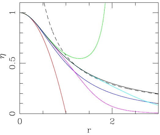
Fig. 1 Dimensionless density vs. dimensionless radius for the exact (numerical) non-singular solution (black, solid line), the second order non-singular solution (red, solid line) and the singular solution (dashed line). The alternative second order solution (blue line), the 4th order solution (green), the 6th order solution (magenta) and the “near field” fit (cyan) described in § 4.1 are also shown. The color figure can be viewed online. 

4. THE LARGE R CONVERGENCE TO THE SINGULAR SOLUTION

As has been done in the past for the non-singular isothermal sphere solution (see, e.g., Chandrasekhar 1964; R2013a), we now study the large r convergence of the non-singular logatropic sphere to the singular solution. In order to do this, we define a function q(r) such that:

where η(r) is the non-singular solution of equation (10) and η_S(r) is the singular solution (equation 12).

We substitute equation (13) in both sides of equation (10), and assuming that q, dq/dr, d²q/dr² ≪ 1, we only keep the terms that depend linearly on q and its derivatives. This exercise results in the differential equation:

Assuming a solution of the form q ∝ r^p and substituting into equation (14) one obtains an exponent p=(-3±7i)/2. Then, the real part of the solution

where B and φ are integration constants. This oscillating solution at large radii has the same period (in lnr) as the one found for the isothermal sphere (see equation 15 of R2013a). Nevertheless, the amplitude decreases much faster with radius, like r^−3/2, rather than the slower r^−1/2 dependence obtained for the isothermal sphere.

5. AN APPROXIMATE ANALYTIC SOLUTION

In this section we present an analytic approximation for the density η(r) over the whole 0 < r < ∞ interval.

5.3. The Full Approximate Analytic Solution

We propose an approximate analytic solution for all r given by:

ηa(r)={ηnear(r);forr≤1,ηfar(r);forr>1. (22)

The top panel of Figure 2 shows the logarithm of the dimensionless density η versus the logarithm of radius r for the exact (numerical) solution and the approximate near/far field solution of equation (22). Both solutions are indistinguishable at the resolution of the figure. The middle panel shows the difference between the exact (numerical) non-singular solution and the singular solution, q = η/η_S−1, as a function of r (see equation 13). Again, the results obtained with the exact and approximate analytic solutions are indistinguishable. Only the first oscillation of the far-field solution appears because the rest are attenuated by the factor r ^−3/2 (see Figure 4 below). The relative deviation (η_α − η)/η of the analytic approximation η_α from the exact (numerical) non-singular solution is plotted as a function of r in the bottom panel of Figure 2. It is clear that the errors in η_a are smaller than ≈ 0.2% for all r. Because of this, at the resolution of the top panels of this figure, the analytic approximation is indistinguishable from the exact (numerical) solution.

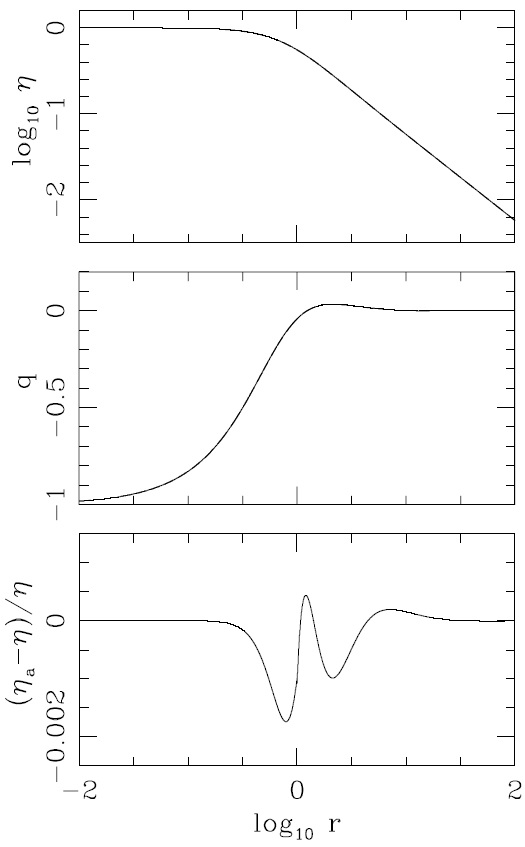
Fig. 2 Top: density vs. radius for the exact (numerical) non-singular solution (solid line). Center: deviation q = η/η_S − 1 (see equation 13) of the exact solution from the singular solution. Bottom: deviation η_α/η− 1 between the full near/far field analytic approximation (equation 22) and the exact numerical solution. In the two top frames we have also plotted the results obtained using η_a (instead of the exact solution, as dashed lines), but at the resolution of the plots they are indistinguishable from the solid curves corresponding to the exact solution. 

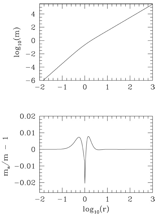
Fig. 3 The solid line in the upper panel shows the exact (numerical) mass m(r) and the dotted line shows the analytic mass m _α(r) obtained from equation 25. The lower panel shows the fractional difference between the analytic and exact (numerical) masses, (m _α−m)/m, where the modulus is always smaller than 0.02. 

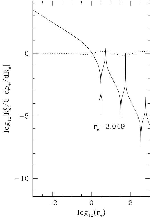
Fig. 4 The solid line shows the logarithm of the absolute value of the stability criterion in equation (38) obtained with the exact (numerical) solution η(r), and the dotted-dashed line shows the derivative calculated with the analytic solution η_α(r). Note that the cusps extend to ±∞ when the argument of the logarithm goes through zero. The dotted line shows r ^3/2q, where q = η/η_S − 1 is the fractional deviation of the dimensionless density with respect to the singular solution. 

6. STABILITY TO RADIAL PERTURBATIONS

The radial stability analysis of the isothermal self-gravitating finite gas sphere was done by ^{Bonnor (1956)} and ^Ebert(1957) who showed that there is a maximum radius for an isothermal sphere to be stable to gravitational collapse. ^{Bonnor (1956)} proposed the criterion for stability of a finite isothermal self-gravitating gas sphere with radius R _e and total mas M against radial perturbations,

In the case of a logatropic sphere, this criterion becomes:

where ρ _e = ρ(R_e). ^{McLaughlin and Pudritz (1996)} calculated the stability of the logatropic sphere assuming that the singular solution was valid at the external radius r_e (see their equation 4.6). Here we calculate this criterion from the exact (numerical) and analytic solutions (the latter given by equation 22) following ^{Raga et al. (2013b)}, who calculated the stability of an isothermal gas sphere to radial perturbations.

In dimensional units one can write the logatropic density at the external radius R_e as:

and the dimensional mass inside a radius R_e as:

where r _e = R_e/R_c, m(r) is given by Equation (24), and we have used Equation (8) for the core radius R_c.

One wants to consider radial perturbations of a sphere at constant mass. First, one differentiates Equation (29), obtaining:

where, from equation (24),

Setting dM = 0 and substituting ∂r_e/∂R_c = −r_e/R_c, ∂r_e/∂R_e = 1/R_c, one obtains:

Therefore, for radial variations at constant mass, one can write the derivative of the core radius with respect to the external boundary as:

The criterion for stability is dρ_e/dR_e > 0 (see equation 27). In the logatropic sphere, this derivative is:

where we have used equation (34) and

Substituting m(r) in equation (25), the criterion for stability of the logatropic sphere against radial perturbations is:

The logarithm of the absolute value of this derivative is shown in Figure 4 where the solid line is obtained with the exact (numerical) solution η(r) and the dotted-dashed line is obtained with the analytic solution η_a(r) of equation (22). Both lines almost coincide. The arrow shows the dimensionless critical radius for stability:

where the derivative becomes negative. This is the maximum external radius for which one has a gravitationally stable configuration. In the notation of ^{McLaughlin & Pudritz (1996}), r_crit corresponds to ξ_crit = R_crit/r₀ = (2A/3)^1/23.049, where A is their pressure parameter defined in their equation (4.1), and r₀ = (3/2A)^1/2R_c is their scale radius. Our value of the critical radius (or ξ_crit) differs from the value they obtained in their equation (4.6), ξcritMP=(2A/9)1/2exp⁡(1/A-1/4). This difference is due to their use of the singular solution (η_S) to evaluate the stability criterion, and their constraint of a constant velocity dispersion at the center of the sphere. In contrast, we used the exact numerical solution (η) to evaluate the stability criterion, and we kept an invariant P vs. ρ relation (see equation 1), leading to a “heating” of the turbulent motions in the center of the cloud in response to small compressions.

There are other bands of stability with r _e > r_crit where the derivative is positive. These bands are related to the oscillations of η(r) at large radii In order to visualize the oscillations of η(r) at large radii, the dotted line in Figure 4 shows r^3/2 q(r), where q = η/η_S − 1 is the fractional deviation of the dimensionless density with respect to the singular solution of equation (12). Even though one could have a sphere with a larger radius r_e > r_crit where the derivative is positive, ^{Bonnor (1956)} argued that any radial perturbation would eventually reach an unstable inner region, inducing the overall collapse.

Given the critical radius r_crit, the ratio between the central density ρ_c and the density at the cloud edge in a gravitationally stable logatropic sphere is given by:

which is smaller than the value of 14.7 obtained for the case of the isothermal sphere. Furthermore, the ratio of the velocity dispersions at the cloud center and at the cloud edge is σ_c/σ(r_crit) = ρ(r_crit)/ρ_c = 0.192. Also, the Jeans length at the cloud center is λJ=csπ/(Gρc), where the sound speed is cs=σ=P0/ρc . If we define the Jeans radius as R_J = λ_J/2, then the ratio of the cloud critical radius to the Jeans radius is R_crit/R_J = 2(3.049/π)(3/2)^1/2 = 2.38.

7. CONCLUSIONS

We present an approximate analytic solution for the density of the non-singular self-gravitating logatropic gas sphere that differs by less than 0.2% from the exact (numerical) solution. The analytic mass differs by less than 2% from the exact mass. This analytic function η_α (eq. (22) can be useful for the study of this type of clouds.

We calculate the gravitational stability of the logatropic sphere to radial perturbations and find a maximum external radius R_crit = 3.049R_c, where the core radius is expressed in terms of the properties of the logatropic sphere Rc=3P0/(2πGρc2). This value implies a maximum density ratio of the density at the cloud center to the density at the external radius, ρ _c/ρ(r_crit) = 5.2, smaller than the factor of 14.7 which is obtained for the isothermal sphere.