


 text new page (beta)
 English (pdf)
 Article in xml format
 Article references
 Send this article by e-mail
 Cited by SciELO
  Similars in
SciELO
Similars in
SciELO 
 Permalink
1. INTRODUCTION
Isothermal models play an important role in many astrophysical problems, in particular in stellar structure and galactic dynamics (Chandrasekhar 1939; Binney & Tremaine 1987; Rose 1998; Chavanis 2002, 2008). Regarding stellar structure and evolution theory, one can obtain the behavior of the physical variables through the isothermal self-gravitating spheres. In the equation of state P = Kρ 1+1/n (where P is the pressure, ρ is the density and K is the polytropic constant), the polytropic index n ranges from 0 to ∞ (Liu 1996; Mirza 2009). In galactic dynamics, the polytropic index n is larger than 0.5 and the Lane-Emden equation for isothermal configurations is considered as a generating function of potential models for flattened galactic systems (Binney & Tremaine 1987).
In the framework of Newtonian mechanics (nonrelativistic), isothermal spheres have been much investigated by many authors (Milgrom 1984; Liu 1996; Natarajan & Lynden-Bell 1997; Roxburgh & Stockman 1999; Hunter 2001; Nouh 2004; Mirza 2009; Raga et al. 2013). In the framework of the theory of general relativity, numerical studies on the relativistic isothermal spheres were performed by several authors (Edward & Merilan 1981a,b; Zhang et al. 1983; Chavanis 2002, 2008; Chau et al. 1984). (Chau et al. 1984) extended the work done by Edward & Merilan (1981a,b) to determine the static structure of general relativistic, partially degenerate, isothermal (with arbitrary temperature) configurations. Chavanis (2002, 2008) investigated the structure and stability of isothermal gas spheres in the framework of general relativity with a linear equation of state P = qє (є: the mass-energy density, P: pressure and q → 0 for Newtonian gravity). Sharma (1990) introduced approximate analytical solutions to the TOV equation of hydrostatic equilibrium in a concise and simple form using a Pad´e approximation technique. His results show that general relativity isothermal configurations are of finite extent. The geometrical size derived by Sharma (1990), ξ = ξ1, for the configurations is limited to ξ1 = 2.
Due to the lack of a full analytical solution to the TOV equation of hydrostatic equilibrium and the importance of the study of relativistic isothermal configurations for various astronomical objects, we introduce a new approximate analytical solution to the Tolman-Oppenheimer-Volkoff (TOV) equation based on a combination of the two techniques: the Euler-Abel transformation and the Pad´e approximation (Nouh & Saad 2013). The constructed analytical solution is in a general form such that we can increase the number of terms of the series solution for the desired accuracy. We display the solution curves in the ξ-θ and ξ-ν phase planes for three general relativistic effects σ = 0.1, 0.2 and 0.3. The proposed method is promising and can examine efficiently the behavior of the physical parameters of stars, such as density, pressure, temperature, etc. from the center towards the surface.
2. FORMULATIONS
The Tolman-Oppenheimer-Volkoff equation of the isothermal gas sphere could be given by Sharma (1990).
where Mr is the total mass energy or “effective mass” of the star of radius r including its gravitational field, that is,
Define the variables, ξ, θ, ν and the relativistic parameter σ by the following equations.
where ρ c and Pc define the central density and central pressure of the star respectively. ν is the mass function of radius ξ , and c is the speed of light. Equations (1) and (2) can be transformed into the dimensionless forms in the (ξ, θ) plane as:
which satisfy the initial conditions
If the pressure is much smaller than the energy density at the center of a star (i.e. σ tends to zero), the non-relativistic case, then the systems (5) and (6) reduce to yield the classical non degenerate isothermal structure equations (Chandrasekhar 1939)
3. SERIES SOLUTION
Equation (5) can be written in the form
Consider a series expansion near the origin ξ = 0 , of the form
that satisfies the initial conditions (7); at θ(0) = 0 yields α0 = 0; then
Multiplying equation (11) by ξ2 yields
With the help of some algebraic operations on series (Nouh and Saad 2013), we get:
Inserting Equation (9) in Equation (6) yields
Integrating both sides of the last equation gives
Multiplying both sides of equation (12) by ν and using equation (16)we obtain:
Let
then
Implementing the formula of multiplication of two series(Nouh & Saad 2013), Equation (19) becomes:
where
Substituting equations (13),(14),(16) and (20) in equation (9) yields:
that is,
Then, the series coefficients formula has the form:
where
For example, the coefficient a1 can be computed from
Considering σ = 0 in equation (18), we get
4. RESULTS
The analytical solution of equations (5) and (6) with the given initial conditions in equation (7) determines the relativistic structure of the configuration. This solution is represented by equation (10) together with equations (23) to (25). The radius of convergence ξ1 of the power series solution without applying any acceleration techniques is limited. Tables 1, 2 and 3 show the solutions θ(ξ1), the mass function ν(ξ1) and the errors between analytical and numerical solutions ε1 and ε2 respectively. It is found that the maximum radii of convergence for the relativistic effects σ = 0.1,0.2 and 0.3 are 3.58, 3.23 and 2.8 respectively. Beyond the mentioned values, the power series solution is either slowly convergent or divergent. It is worth noting that we have used the fourth order Runge-Kutta method for the numerical solution of the TOV equation.
Table 1 Radius of convergence of the power series solution of the tov equation for the relativistic effect σ = 0.1 before acceleration
| ξ | θ(ξ1)-An | Error(ξ1) | ν(ξ1)-An | Error(ξ2) |
| 0.1 | 0.0023821620 | −1.0260393175E − 006 | 0.0003328572 | 3.7246274503E − 009 |
| 0.3 | 0.0213554534 | −8.7300804448E − 007 | 0.0088854114 | 2.7700080786E − 008 |
| 0.5 | 0.0588588473 | −8.2433308801E − 007 | 0.0402206825 | 4.3356597944E − 008 |
| 0.7 | 0.1140289083 | −7.7062136704E − 007 | 0.1067702316 | 6.2923817407E − 008 |
| 1.0 | 0.2271109903 | −6.7723700739E − 007 | 0.2908362576 | 2.0858204730E − 007 |
| 1.5 | 0.4823843992 | −4.7763943689E − 007 | 0.8415768047 | 3.5292719458E − 007 |
| 2.0 | 0.7949739993 | −2.5950480864E − 007 | 1.6496506598 | 8.9354771737E − 007 |
| 2.5 | 1.1356472829 | −1.1575548076E − 007 | 2.6113910910 | 9.6941780958E − 007 |
| 3.0 | 1.4811590655 | −4.6188424359E − 006 | 3.6301217015 | 1.1506687414E − 005 |
| 3.2 | 1.6165050544 | −0.00051449094 | 4.0396568830 | 0.0014489918 |
| 3.4 | 1.7076830315 | −0.04276749508 | 4.5893860584 | 0.1469808356 |
| 3.5 | 1.4627148414 | −0.35338134721 | 5.9789554323 | 1.3365109770 |
Table 2 Radius of convergence of the power series solution of the tov equation for the relativistic effect σ = 0.2 before acceleration
| ξ | θ(ξ1)-An | Error(ξ1) | ν(ξ1)-An | Error(ξ2) |
| 0.1 | 0.0031982938 | −2.2362586831E − 006 | 0.0003326943 | −2.9907271354E − 008 |
| 0.3 | 0.0286620788 | −2.2502026265E − 006 | 0.0088465883 | 2.16251607697E − 008 |
| 0.5 | 0.0789402709 | −2.1395188244E − 006 | 0.0397404600 | 8.08164897295E − 008 |
| 0.7 | 0.1527556329 | −1.9796703668E − 006 | 0.1043317478 | 2.06352842008E − 007 |
| 1.0 | 0.3034042901 | −1.6674736475E − 006 | 0.2779523918 | 5.19178451952E − 007 |
| 1.5 | 0.6393200909 | −1.0088775712E − 006 | 0.7670949161 | 1.16339283773E − 006 |
| 2.0 | 1.0404738378 | −3.5765433481E − 007 | 1.4268048236 | 1.69882056111E − 006 |
| 2.5 | 1.4623116228 | −2.6108234761E − 006 | 2.1481527204 | 3.96874110464E − 006 |
| 3.0 | 1.8307363050 | −0.0417696517 | 2.9183335680 | 0.05979638685 |
| 3.1 | 1.7175597721 | −0.2337994006 | 3.3725656715 | 0.37656844720 |
| 3.2 | 0.7921498711 | −1.2367731914 | 5.3648422145 | 2.23325307786 |
Table 3 Radius of convergence of the power series solution of the tov equation for the relativistic effect σ = 0.3 before acceleration
| ξ | θ(ξ1)-An | Error(ξ1) | ν(ξ1)-An | Error(ξ2) |
| 0.1 | 0.0041140941 | −2.3715336048E − 006 | 0.0003325116 | −2.5482476363E − 008 |
| 0.3 | 0.0368418883 | −2.4174640616E − 006 | 0.0088033324 | 1.72283842661E − 008 |
| 0.5 | 0.1013152851 | −2.3181737671E − 006 | 0.0392122892 | 6.73057481138E − 008 |
| 0.7 | 0.1955935387 | −2.1051340775E − 006 | 0.1017001108 | 1.81159963003E − 007 |
| 1.0 | 0.3864665335 | −1.6654161666E − 006 | 0.2645710374 | 5.02286165494E − 007 |
| 1.5 | 0.8034447178 | −8.0623353149E − 007 | 0.6959310510 | 1.12674301400E − 006 |
| 2.0 | 1.2834657367 | 7.36378646948E − 009 | 1.2331174045 | 1.38017677043E − 006 |
| 2.5 | 1.7667238793 | 0.00088563654 | 1.7804026764 | −0.0005676831 |
| 2.6 | 1.8657341938 | 0.00682973775 | 1.8819879809 | −0.0051201240 |
| 2.7 | 1.9989280051 | 0.04858109323 | 1.9493098672 | −0.0423219728 |
| 2.8 | 2.3605847415 | 0.32055375109 | 1.7713173023 | −0.3231297424 |
Therefore, it was necessary to improve the power series solution of the TOV relativistic equation, which in turn contributes to obtain a better approximation to the physical parameters of stars. A combination of the two techniques for the Euler-Abel transformation and the Pad´e approximation (Nouh 2004; Nouh & Saad 2013) has been utilized. Figures 1, 2 and 3 represent the solution curves of the TOV equation in the ξ-θ phase plane for the general relativistic effects σ = 0.1,0.2 and 0.3, respectively. Each figure displays both analytical (dashed line) and numerical (solid line) solutions and their relative error. The maximum relative error was of order 10−3 for σ = 0.1,0.2, while for σ = 0.3 the relative error was of order 10−2. In the same way, Figures 4, 5 and 6 show the solution curves in the ξ-ν phase plane for the general relativistic effects σ = 0.1,0.2 and σ = 0.3 respectively. When comparing the accelerated solution with the numerical one, we found that the series tends to converge slowly for ξ > 20. The most important finding is that the physical range of the convergent power series solutions extended to around ten times that of the classical procedures.
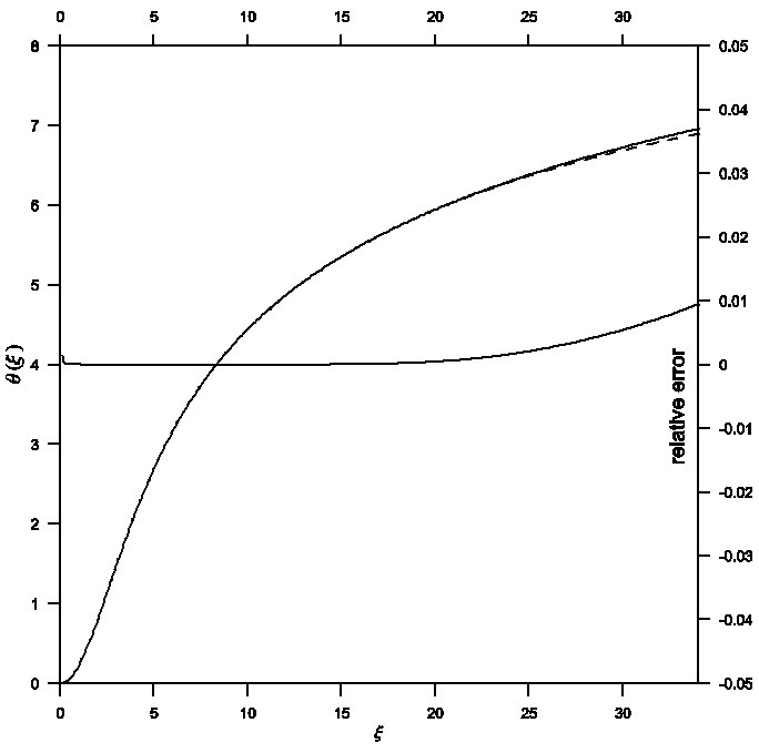
Fig. 1 Solution of the TOV equation in the ξ-θ phase plane for general relativistic effect σ = 0.1. Comparison between analytical (dashed) and numerical (solid) solutions gives a maximum relative error of order 10−3.
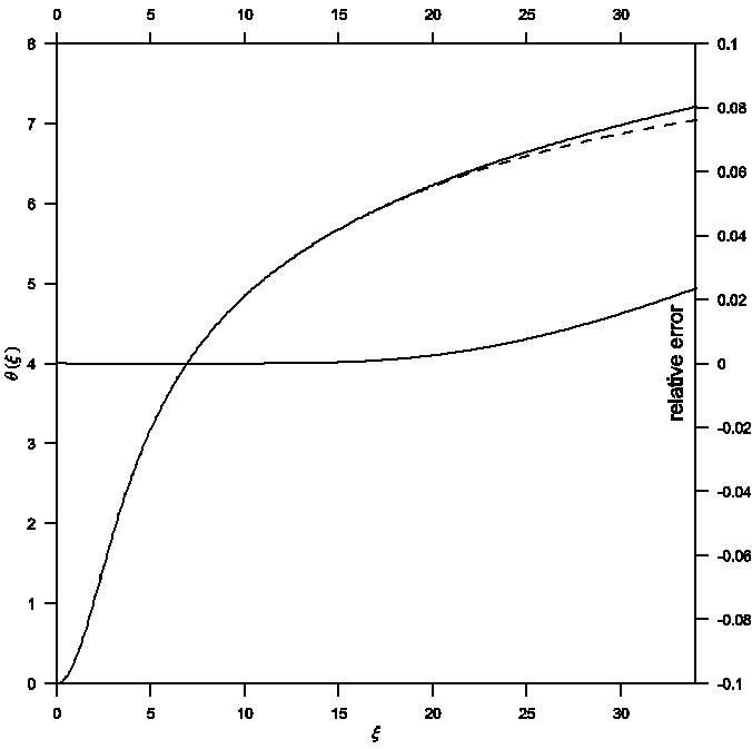
Fig. 2 Solution of the TOV equation in the ξ-θ phase plane for general relativistic effect σ = 0.2. Comparison between analytical (dashed) and numerical (solid) solutions gives a maximum relative error of order 10−3.
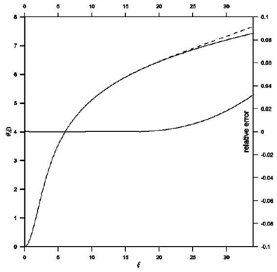
Fig. 3 Solution of the TOV equation in the ξ-θ phase plane for general relativistic effect σ = 0.3. Comparison between analytical (dashed) and numerical (solid) solutions gives a maximum relative error of order 10−2.
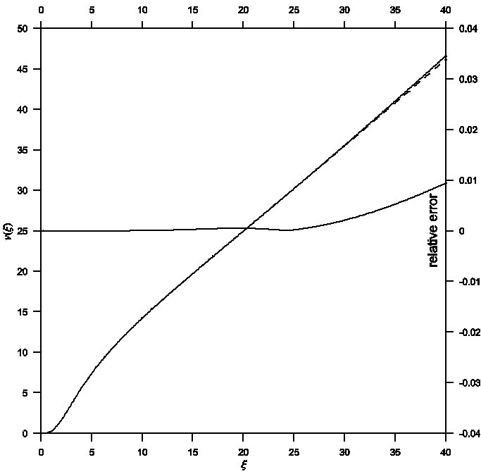
Fig. 4 Mass function ν(ξ) in the ξ-ν phase plane for general relativistic effect σ = 0.1. Comparison between analytical (dashed) and numerical (solid) solutions gives a maximum relative error of order 10−3.
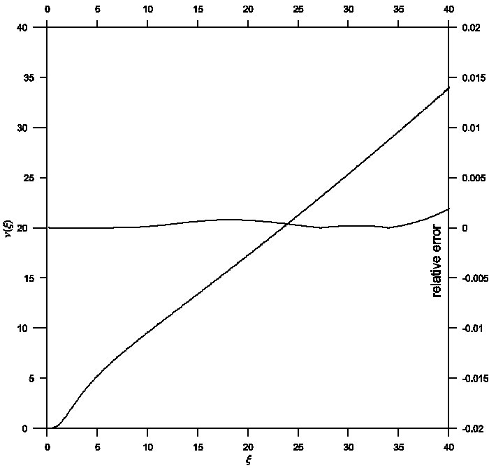
Fig. 5 Mass function ν(ξ) in the ξ-ν phase plane for general relativistic effect σ = 0.2. Comparison between analytical (dashed) and numerical (solid) solutions gives a maximum relative error of order 10−3.
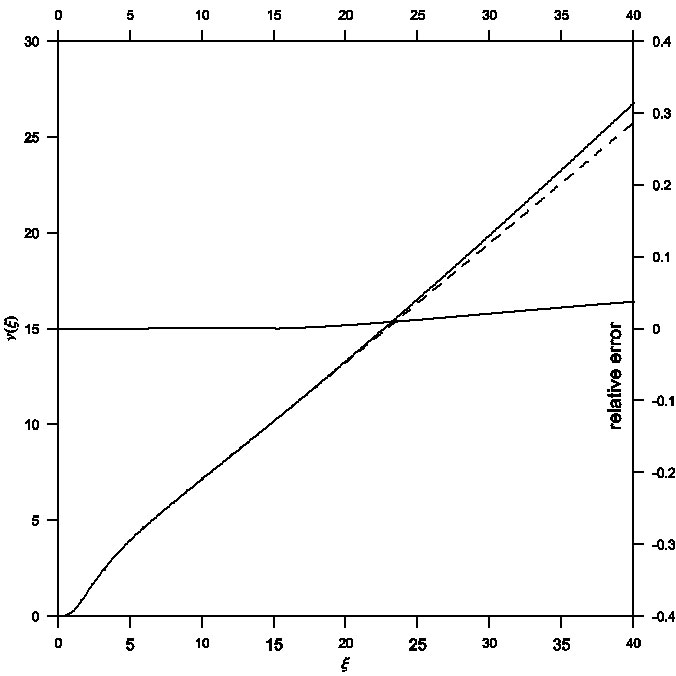
Fig. 6 Mass function ν(ξ) in the ξ-ν phase plane for general relativistic effect σ = 0.3. Comparison between analytical (dashed) and numerical (solid) solutions gives a maximum relative error of order 10−2.
4.1. Application to Neutron Stars
The aim of the study of stellar structure, either in the framework of Newtonian mechanics (nonrelativistic) or in the framework of general relativity (relativistic) is to investigate and examine the behavior of the physical parameters, such as pressure, density, temperature, mass, etc., and to determine the mass-radius relation.In this context, the proposed analytical solution in the present paper was applied to a neutron star with the physical parameters: mass M = 1.5M⊙, central density ρc = 5.75 × 10¹⁴ gcm−3, pressure P = 2 × 1033 par, and radius R = 1.4×106 cm. Tables 4, 5 and 6 show the physical parameters of a neutron star obtained from a direct analytical solution of the TOV equation with the relativistic isothermal configurations σ = 0.1, 0.2 and 0.3. The tables give the mass ratio M/M0 in the first column and the error between analytical and numerical ε1, while Columns 3 and 4 show the density ratio ρ/ρc and its error ε2. The error is increasing gradually and the radius of convergence of the power series solution is limited. Therefore, the calculated physical parameters have poor accuracy.
Table 4 Physical parameters of a neutron star before accelerating the power series solution with the relativistic isothermal configuration σ = 0.1
| ξ | M/M0-An | Error(ξ1) | ρ/ρc-An | Error(ξ2) |
| 0.1 | 6.50157995E − 005 | −7.93658100E − 006 | 0.99762067 | 1.02359751E − 006 |
| 0.3 | 0.00173556 | −0.00021188 | 0.97887096 | 8.54561849E − 007 |
| 0.5 | 0.00785616 | −0.00095910 | 0.94283984 | 7.77213760E − 007 |
| 0.7 | 0.02085504 | −0.00254606 | 0.89223216 | 6.87572904E − 007 |
| 1.0 | 0.05680799 | −0.00693531 | 0.79683234 | 5.39644164E − 007 |
| 1.5 | 0.16438215 | −0.02006837 | 0.61730972 | 2.94851398E − 007 |
| 2.0 | 0.32222029 | −0.03933779 | 0.45159298 | 1.17190534E − 007 |
| 2.5 | 0.51007357 | −0.06227168 | 0.32121414 | 3.71822947E − 008 |
| 3.0 | 0.70905853 | −0.08656227 | 0.22737399 | 1.05020223E − 006 |
| 3.2 | 0.78905155 | −0.09601309 | 0.19859155 | 0.00010215 |
| 3.4 | 0.89642816 | −0.07722548 | 0.18128534 | 0.00758967 |
| 3.5 | 1.16784772 | 0.150350954 | 0.23160665 | 0.06894714 |
Table 5 Physical parameters of a neutron star before accelerating the power series solution with the relativistic isothermal configuration σ = 0.2
| ξ | M/M0-An | Error(ξ1) | ρ/ρc-An | Error(ξ2) |
| 0.1 | 1.84156019E − 010 | −5.01634030E − 012 | 0.99999968 | 3.01749311E − 008 |
| 0.3 | 0.00148393 | −1.90493760E − 009 | 0.98718236 | 2.24118632E − 006 |
| 0.5 | 0.01151679 | 6.649477030E − 009 | 0.95026265 | 2.08770747E − 006 |
| 0.7 | 0.03735025 | 3.813366056E − 008 | 0.89281237 | 1.84370015E − 006 |
| 1.0 | 0.11605026 | 2.927041631E − 008 | 0.77975328 | 1.39542662E − 006 |
| 1.5 | 0.36081190 | 9.344106428E − 008 | 0.56773599 | 6.57116908E − 007 |
| 2.0 | 0.71167074 | 1.328278937E − 007 | 0.38361304 | 1.87786358E − 007 |
| 2.5 | 1.10745911 | 7.846480399E − 008 | 0.25185372 | 4.60871126E − 008 |
| 3.0 | 1.50812170 | 0.005015086 | 0.16761343 | 0.00119469 |
| 3.1 | 1.61367473 | 0.033657910 | 0.16028642 | 0.00667063 |
| 3.2 | 1.86778757 | 0.211838462 | 0.18008080 | 0.03811105 |
Table 6 Physical parameters of a neutron star before accelerating the power series solution with the relativistic isothermal configuration σ = 0.3
| ξ | M/M0-An | Error(ξ1) | ρ/ρc-An | Error(ξ2) |
| 0.1 | 3.38314717E − 010 | −6.88539237E − 012 | 0.99999959 | 2.92341651E − 008 |
| 0.3 | 0.00272011 | −9.11526077E − 009 | 0.98354708 | 2.44318533E − 006 |
| 0.5 | 0.02097454 | 1.422439966E − 008 | 0.93656827 | 2.23634834E − 006 |
| 0.7 | 0.06731848 | 4.124582367E − 008 | 0.86471217 | 1.91681736E − 006 |
| 1.0 | 0.20465838 | 1.439727668E − 007 | 0.72796240 | 1.32236526E − 006 |
| 1.5 | 0.60732845 | 2.002381181E − 007 | 0.48984974 | 4.83381012E − 007 |
| 2.0 | 1.14039429 | −1.15562337E − 007 | 0.30525537 | 4.27123615E − 008 |
| 2.5 | 1.69940711 | −6.07445250E − 005 | 0.18780008 | −2.0258932E − 005 |
| 2.6 | 1.80808156 | −0.000591672 | 0.17072850 | −0.0001545 |
| 2.7 | 1.91106920 | −0.005312332 | 0.15461843 | −0.0010811 |
| 2.8 | 1.97859450 | −0.043856014 | 0.13523016 | −0.0068658 |
| 2.9 | 1.79221566 | −0.334569026 | 0.09371845 | −0.0361909 |
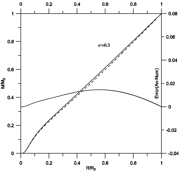
On the other hand, manipulation of the analytical solution by means of the proposed procedure improved the solution, which of course will be reflected on the accuracy of the estimated physical parameters. Figures 7, 8 and 9 describe the density profile for isothermal spheres with relativistic effects σ = 0.1,0.2 and 0.3. As shown, the density decreases with increasing radius of the star. In all the figures the analytical and numerical curves cannot be distinguished. A comparison between analytical (solid) and numerical (dashed) solutions gives a maximum relative error of order 10−4. Figures 10, 11 and 12 plot the analytical and numerical values of the ratios M/M0 and their errors.
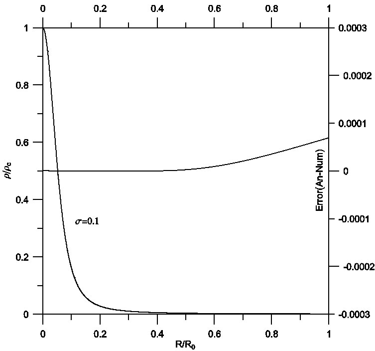
Fig. 7 Density profile for isothermal spheres with relativistic effects σ = 0.1. Comparison between analytical (solid) and numerical (dashed) solutions gives a maximum relative error of order 10−4.
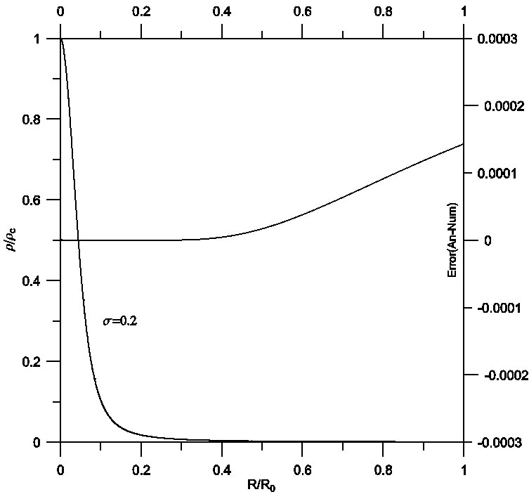
Fig. 8 Density profile for isothermal spheres with relativistic effects σ = 0.2. Comparison between analytical (solid) and numerical (dashed) solutions gives a maximum relative error of order 10−4.
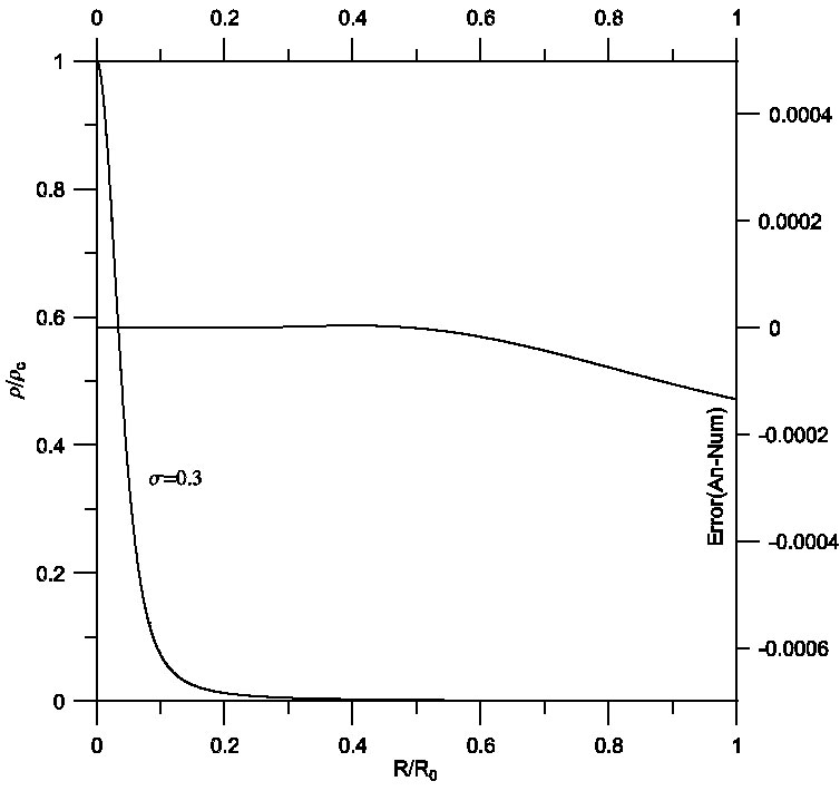
Fig. 9 Density profile for isothermal spheres with relativistic effects σ = 0.3. Comparison between analytical (solid) and numerical (dashed) solutions gives a maximum relative error of order 10−4.
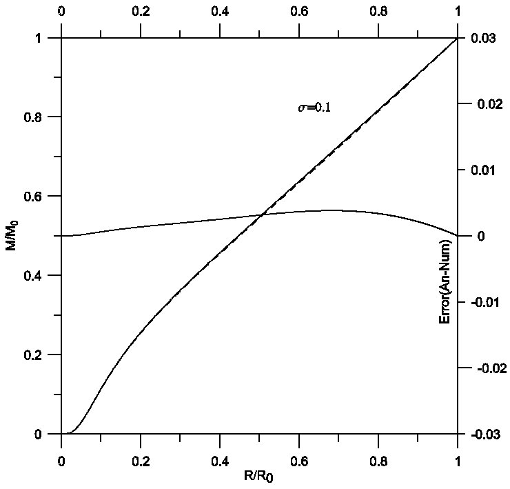
Fig. 10 Mass profile for isothermal spheres with relativistic effects σ = 0.1. Comparison between analytical (solid) and numerical (dashed) solutions gives a maximum relative error of order 10−3.
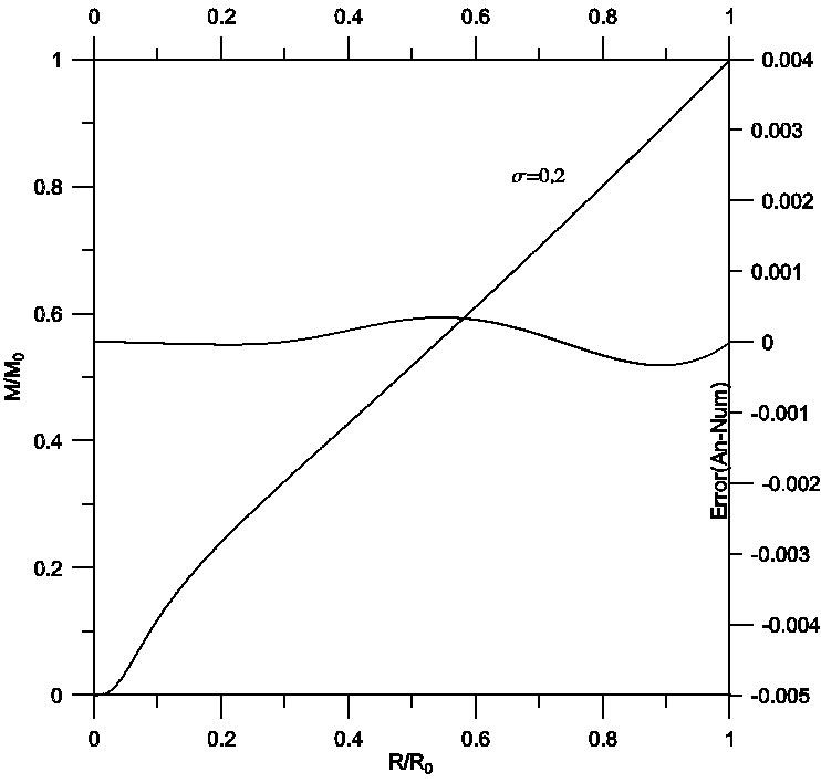
Fig. 11 Mass profile for isothermal spheres with relativistic effects σ = 0.2. Comparison between analytical (solid) and numerical (dashed) solutions gives a maximum relative error of order 10−3.
5. CONCLUSIONS
We have constructed general analytical formulations for solving the hydrostatic equilibrium equation (TOV equation) in the framework of relativistic isothermal gas spheres. Traditional procedures for its solution were not effective and the radius of convergence of the power series solution was limited, as shown in Tables 1, 2 and 3. That is, the maximum radii of convergence for the relativistic effects σ = 0.1,0.2 and 0.3 were ξ1 = 3.58, ξ1 = 3.23 and ξ1 = 2.8, respectively. When we improved the power series solution utilizing a combination of the two techniques: an Euler-Abel transformation and a Padé approximation (Nouh 2004; Nouh & Saad 2013), the radius of convergence increased. As a result, the physical range of the convergent power series solutions was extended to about ten times that of the traditional procedures (ξ1 ≈ 35), as displayed in Figures 1, 2 and 3. The implementation of the proposed analytical solution contributed to improve the accuracy of the calculation of the physical parameters of the stars. As shown in Figures 7 to 12 for the density and mass profiles of the star, the maximum relative error reached 10−3, which establishes the validity and accuracy of the suggested procedure. The analytical solution derived in the present paper may be a good contribution to the field of stellar structure.

