1. Introduction

The Great comet of 1819 (C/1819 N1), also known as Comet Tralles, discovered on 2 July 1819 and followed until 15 October of that year was the first comet to be observed with polarimetry (^{Kolokolova, Hough & Levasseur-Regourd 1999, p.380}). It also has the distinction of being a visual comet that transited the sun, on 26 June, shortly before discovery (^{Hind 1876}). Hind also discusses whether the transit was actually observed rather than thought to be observed; on the day of the transit no one knew that an actual comet was passing over the solar surface.

Because the orbit contained in the ^{Marsden and Williams catalog (2003)} and the JPL Small-Body Database Browser (http://ssd.jpl.nasa.gov/sbdb.cqi) was calculated in 1906 (^{Peck 1906}), to recompute the orbit by use of modern computing techniques and statistical analysis seems a worthwhile endeavor. Peck concluded that the orbit was indistinguishable from a parabola (^{Peck 1907}), but seeing as he based his analysis on normal places, a computational expediency almost necessary a century ago but deleterious nevertheless, this conclusion must be checked against what modern computing has to say.

2. The observations and their treatment

Because it was discovered before standard journals such as Monthly Notices and Astronomische Nachrichten were founded, observations of the Great comet are difficult to obtain. Many are contained in sources such as the Berliner Jahrbuch and in the annals of various observatories not available in the ADS database (http://adswww.harvard.edu/). Fortunately, ^{Peck (1906)} published a list of all of the observations, 402 in right ascension (α) and 294 in declination (δ). Because the comet was bright, many observations, 135 in α and 106 in δ were made by meridian instruments. Peck also managed to identify individual reference stars for some of the non-meridian observations. He lists 29 reference stars referred to the equinox of 1819. Of these 29 I was able to find all but 3 in the Tycho-2 catalog (^{Høg et al. 2000}). Therefore, 100 of the observations could be corrected for the difference between the Tycho-2 catalog, presumably more precise, and Peck’s reference star list. All observations must be corrected for the astronomical-civil day difference and also for the difference between Greenwich mean time and terrestrial time. Nor will the observations be formed into normal places, but rather used directly.

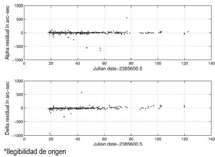
Fig. 1 graphs the observations, and Table 1 shows their distribution among observatories. Table 1 gives no references because ^{Peck (1906)} identifies the sources for all of the observations.

Fig. 1 The observations. 

3. Ephemerides and differential corrections

The procedure for calculating coordinates, velocities, and partial derivatives for differential corrections has been given in previous publications of mine. See ^{Branham (2005)}, for example. The first differential correction was based on the robust L₁ criterion, minimize the sum of the absolute values of the residuals, insensitive to discordant data, and leaving 696 equations of condition.

Various weighting schemes are possible once one has post-fit residuals from a differential correction. Modern schemes assign higher weight to smaller residuals and zero weight to large residuals, recognizing them as errors rather than genuine but improbable residuals. Among these robust weightings I chose the Welsch (^{Branham 1990, Sec. 5.5}), largely because it yields good results with Galactic kinematics; see ^{Branham (2014)}. Welsch weighting accepts all residuals, but assigns low weight to large residuals, so low as to become less than the machine ε for extremely large residuals,

Weights calculated from Eq. (1) were applied to the equations of condition.

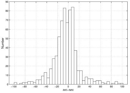
Fig. 2 shows a histogram of the weights. The mean error of unit weight, σ(1), becomes 11.''23, some what high but still in a normal range for 19th century comets; see Table A1 in ^{Branham (2012)}.

Fig. 2 Histogram of Welsch weights. 

4. The solution

Table 2 shows the final solution for the rectangular coordinates, x₀, y₀, z₀, and velocities, x˙ ₀ y˙₀, z˙₀, along with their mean errors and also σ(1) for the comet. Table 3 gives the corresponding covariance and correlation matrices. All correlation are high, the highest being -97.7% between x₀ and y₀. Although statistically significant, these correlations nevertheless do not imply an unstable solution because the condition number of 3.2 x 10² for the data matrix shows that it is far from poorly conditioned. The rectangular coordinates indicate that the orbit is elliptical. Table 4 converts the rectangular coordinates to elliptical orbital elements using the well known expressions linking orbital elements with their rectangular counterparts. The orbit represents a high eccentricity ellipse rather than a parabola. The calculation of the mean errors of the orbital elements proceeds via a modernized version of Rice’s procedure (1902). See ^{Branham (2005)}.

The fact that the calculated orbit is a high eccentricity ellipse actually agrees with Peck’s orbit, which finds an eccentricity of 0.999792±0.000079. In a later publication, however, ^{Peck (1907)} suggests that a parabola represents the observations just as well, and thus a parabola has entered the literature for the orbit of the Great comet. A high eccentricity ellipse, however, is better, as the next section shows.

5. Discussion

To check how good a solution is, one should study the residuals. The residuals from the first L1 solution are plotted in Fig. 3; there are evidently some outliers. Because I have no access to the original observations, I cannot search for a cause for these anomalies. A runs test, a statistic of the randomness of the residuals, measures how often a variable, distributed about the mean, changes sign from plus to negative or negative to positive, the runs, which have a mean for n data points of n/2+1 and a variance of n(n−2)/4(n−1) (^{Wonnacott and Wonnacott 1972, pp. 409-411}). The L₁ residuals evince 362 runs out of an anticipated 348. The probability of randomness becomes 28.9%, sufficient to state that the residuals are indeed random and can be used with equation (1) to calculate weights. Random, but not arising from a normal distribution. Statistics on residuals trimmed to under |0.5∙10-3| radian, leaving 680 residuals, show that the residuals are skewed, coefficient of skewness 0.11 versus 0 for a normal distribution, platykurtic, kurtosis of 1.57 versus 3 for the normal, and with a Q factor 0.36 versus 2.11 for the normal and thus lighter-tailed. Figure 4 shows a histogram of the trimmed L₁ residuals.

Fig. 3 The L1 residuals. 

Fig. 4 Histogram of trimmed L1 residuals. 

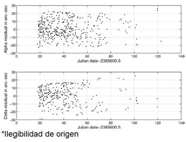
After a new solution has been calculated with the Welsch weights, the solution given in Tables 2 and 4, the statistics change. Fig. 5 plots the residuals from the new solution. A runs test on the non-zero residuals shows 333 runs out of an expected 339, a 64.5% chance of being random. Random, but again non-normal. Statistics on the residuals themselves mean little because the Welsch weighting flattens the distribution and distorts a statistic such as the kurtosis. A mean squared successive difference test (^{Wonnacott and Wonnacott 1972, 411-413}), also known as the Durbin-Watson statistic, measures the serial correlation of one residual with its successor and assumes a normal distribution. For the residuals of Fig. 5 the Durbin-Watson statistic becomes 19.7%, sufficient to infer randomness but with low normality. These statistics show that a high eccentricity ellipse fits the data well.

Fig. 5 Residuals from Welsch weighting. 

Having the orbit the question of whether the Great comet could be a danger to the earth in the future should be answered. The answer is “no.” The Great comet will return to its closest separation from the earth on 18 Feb. 5044, but the separation will be 0.986 AU and thus no threat. It is also interesting to integrate the orbit backwards. On 4 June -2551 the comet passed within 0.790 AU from the earth. This date is close to the time of construction of the Great Pyramid in Egypt. Perhaps some Egyptian chronicles mention a new, bright star in the heavens. Or maybe Sumerian chronicles. This, however, is a question for experts in Near Eastern studies. I merely mention the possibility.

6. The transit of the sun

On 26 June 1819 the Great comet transited the Sun. ^{Hind (1876)} has analyzed supposed observations, or perhaps better stated anomalies on the surface of the Sun because they occurred before it was known that a new comet had been discovered. Of these observations he credits that of Canon Stark as the one most probably identifiable as the comet. Stark observed the solar surface from Augsburg, Germany, and published in his Meteorologisches Jahrbuch that at 7^h 15^m, presumably Augsburg mean time, he saw a remarkable spot 15”25” from the western limb and 14”30” from the northern. When he observed the Sun again at noon the spot had disappeared. I calculate, using the geographical coordinates of Augsburg, that the comet made first contact with the Sun’s limb at 5^h22^m13^s GMT at position angle 171.º 9, last contact at 8h 56m 46m and position angle 9º1, and closest approach of 2”23.”6 at 7^h 8^m 5^s GMT. The Sun’s semidiameter was 15”43.9.

Stark’s measurements imply that the spot he observed was 1”15.”9 from the Sun’s center 31.^m 4 before time of closest approach if we assume that he used Augsburg mean time and more than 1’ closer than the angle of minimum separation. Although these data do not agree closely, the fact that Canon Stark was not a trained astrometric observer (or why would he be publishing in a meteorological journal?) and that the spot he found had disappeared by noon, it seems likely that he indeed saw the comet as it transited the Sun. ^{Hind (1876)} arrives at a similar conclusion. But because of the lack of close agreement between his observation and the data given by computation, the observation unfortunately cannot be used to improve the orbit of the comet.

7. Conclusions

An orbit of the Great comet of 1819 (C/1819 N1) has been calculated by use of 402 observations in α and 294 in δ made between July and October 1819. The orbit is a high eccentricity ellipse. The comet will not return for over 3,000 years and represents no threat to the earth. It is possible that Near Eastern records around 2550 BCE may mention an earlier passage of the Great comet. The comet transited the Sun on 26 June, before the first astronomical observation of 2 July, and was likely seen by at least one observer.