


 text new page (beta)
 English (pdf)
 Article in xml format
 Article references
 Send this article by e-mail
 Cited by SciELO
  Similars in
SciELO
Similars in
SciELO 
 Permalink
1 Introduction
1.1 Background and literature review
It is well known that the nonlinear equation (NLSE) explains the underlying mechanism broadly in numerous fields, such as quantum mechanics [1], plasma physics [2], nonlinear optics [3], optical fibers [4,5], fluid dynamics [6], and hydrodynamics [7]. The related research of the NLSE has mainly focused on their results in fiber optic communication systems. Kundu-Mukherjee-Naskar (KMN) equation is one of the equations that explain the hidden phenomena in the aforementioned fields. More specifically, the KMN equation can be used in fiber amplifiers, optical fiber, data transmission, and so on. Recently, many scholars have studied the different forms of the NLSE about Kerr and non-Kerr law nonlinearities to study optical soliton by using powerful techniques, such as the modified simple equation method [8], the sine-Gordon expansion method [9], the extended simple equation method [10], the modified analytical method [11], the modified Kudryashov method [12] and so on.
In 2013, Kundu and Mukherjee [13] studied the integrable higher-dimensional NLSE and described its features, solutions, and applications. One year later, the KMN equation was first introduced by Kundu et al. [14], which is a new extension of the NLSE (See in section 1.3). The KMN model is the most important model for describing the rough ocean waves and noticeably (2+1)-dimensional characteristics. This model can also be used to propagate light waves through coherently excited resonant waveguides, especially in the case of bending light [15]. Moreover, this model can be useful for the learning of isolated pulses in the (2+1)-dimensional equation [16]. Recently, many scholars have been addressed the exact solutions of the KMN model by using different techniques, such as the first integral method [17], the method of undetermined coefficients and Lie symmetry [18], the trial equation technique [19], the modified simple equation approach [20], the new extended algebraic method [21], the ansatz approach and the sine Gordon expansion method [22], the F-expansion and functional variable methods [23], the new extended direct algebraic method [24], and the exp-function method [25]. Very recently, Kumar et al. [26] discussed the effects of fractional parameters and wave obliqueness of the KMN model by analyzing the soliton pulses, obtained via the generalized Kudryashov and the new auxiliary equation methods. It is noteworthy to mention here that dark, bright, singular, singular period, rough wave, bell, anti-bell type soliton solutions are reported in the previous literature. However, the impacts of wave dispersion and nonlinearity parameters on soliton pulses of the KMN model have not been investigated, as well as the unified method applications’ to the KMN equation.
1.2 Objective of the study
The main goal of this research is to apply the unified method for exploring some new optical solitons, such as dark, bright, periodic, and singular soliton solutions to an integrable KMN equation, which can be of great significance in the field of fiber optics and optical communications. It is noted to mention here that optical solitons are solitary light waves that hold their form over an expansive interval, which produce crystal clear phone calls cross-country and internationally. Furthermore, we will also explain the impacts of wave dispersion and nonlinearity on the attained soliton pulses of the KMN model.
1.3 Mathematical model
In this study, we consider the following (2+1) dimensional KMN equation [14-26] as
In Eq. (1), the spatial variables are represented by x and y, the time variable stands on t, the dependent variable u(x, y, t) is the nonlinear wave envelope and u*(x, y, t) is represented by the complex conjugate of u(x, y, t). The second term in Eq. (1) represents the evolution of the wave followed by the wave dispersion term that is given by the coefficient of σ.
The constant κ ensures the existence of the different case of nonlinearity media which does not fall into the conventional Kerr law nonlinearity or any known non-Kerr law media [16]. The nonlinear term in this equation accounts for “current-like” nonlinearity that stems from chirality [20]. The utmost significant feature of the (2+1)-dimensional KMN model is that it has been given as a new extension of the nonlinear Schrödinger (NLS) equation with the inclusion of different forms of nonlinearity with regard to Kerr and non-Kerr law nonlinearities to study soliton pulses.
1.4 Arrangement of the study
The rest of the paper is organized as follows: the overview of the unified method is presented in Sec. 2. Mathematical analysis is presented in Sec. 3. Graphical analysis of the obtained solutions and the impacts of wave dispersion and nonlinearity on soliton pulses are discussed in Sec. 4. Finally, we give a general conclusion in Sec. 5.
2 Overview of the unified method
The unified method [27,28] is the amalgamation of all hyperbolic tangent function methods, such as the tanh-function scheme, the extended tanh-function technique, the modified extended tanh-function method, and the complex tanh function scheme. In [28], Gozukizil et al., explored the analytic solution to the Rabinovich wave equation and compared between the family of tanh function method and unified method. Besides, they compared the tanh method [29-31], the extended tanh method [32], the modified extended tanh method [33], and the complex tanh-function method [34] with results generated with the unified method. Later, Akcagil and Aydemir [34] applied the unified method to the Lonngren wave equation. They proved that the unified method gives many more general solutions in an elegant way than the family of the tanh-function methods [29-31] and the family of (G’/G)-expansion method, and the (G’/G, 1/G)-expansion method. Besides the unified method, many other methods have been applied for obtaining analytic solutions for NLEEs, such as the (G’/G 2)-expansion method [35], the Hirota bilinear method [36,37], the sine-Gordon equation method [38], the extended sinh-Gordon equation expansion method [39], the enhanced (G’2/G)-expansion method [40,41,42], the exp(-ϕ(ξ)-expansion method [43], the modified simple equation [44], the improved F-expansion method [44], the new ϕ 6-model expansion method [45], the generalized bilinear method [46], the extended Fan sub-equation technique [47], and many more.
The main overviews of the unified method are as follows. Consequently, we consider the general form of the nonlinear partial differential equation as
Using wave transformation
where v is the traveling wave. Inserting Eq. (3) into Eq. (2) yields the following ODE:
Let us consider that Eq. (4) has the following solutions:
where T is the homogeneous balance parameter which can be determined by balancing between highest order linear and nonlinear terms of Eq. (4), and X = X(Ω) satisfies the Riccati differential equation as follow:
where X’ = dX/dΩ, Aj, Bj (j = 1,2,3,…,T) and γ are constants. Eq. (6) has the following solutions:
Cluster 01: If γ < 0, then the hyperbolic function solutions are
Cluster 02: If γ > 0, then the trigonometric function solutions are
Cluster 03: If γ = 0, then the rational function solution is
where
We put Eqs. (5) and (6) in Eq. (4) and associating all the coefficient of Xi = -N ≤ i ≤ N to zero yield a set of algebraic equations for Aj, Bj and γ. Putting Aj, Bj Ω and γ into Eq. (5) and using the general solutions of Eq. (6), it can be obtained the solutions of Eq. (2) directly based on the value of γ.
3 Mathematical analysis
Let us consider the complex wave transformation as follows
In Eq. (16), the amplitude and phase element of the soliton are U(Ω) and ψ(x, y, t) respectively, where Ω = ax -by - vt and ψ = -px - qy + mt +m0. Here, p and q represent the frequencies of the soliton in the x and y directions respectively, whereas m and m0 signifies the wave number and phase of the soliton respectively. In addition, the parameters a and b in Eq. (16) represent the inverse width of the soliton with x and y directions, respectively and v represents the speed of the soliton. Plugging the above transformation into Eq. (1) and equating real and imaginary parts, we attained the following equations:
and
Applying the balance statement on Eq. (17), yields T = 1. So, the solution of Eq. (17) can be expressed in the following form:
Among them A0, A1, and B1 are constant to be determined later and the function X(Ω) satisfies the Eq. (6). Inserting Eq. (19) along with Eq. (6) into Eq. (17) and collecting all terms with the same power of X(Ω) together, equating each coefficient to zero yields a set of algebraic equations in terms of A0, A1, B1 and m. The following solution sets are obtained:
Inserting Eqs. (20)-(22) into Eq. (19) along with the Eqs. (7)-(10), one can attain the following hyperbolic function solutions:
Group one:
where
Group two:
where
Group three:
where
Inserting Eqs. (20)-(22) into Eq. (19) along with the Eqs. (11)-(14), one can attain the following trigonometric function solutions:
Group four:
where
Group five:
where
Group six:
where
Inserting Eqs. (20)-(22) into Eq. (19) along with the Eq. (15), one can attain the rational function solutions.
Group seven:
where
4 Graphical illustrations of the attained solutions
In this section, we will discuss the physical behaviors of the solutions obtained from the KMN equation via some graphical illustrations. The impacts of wave dispersion (σ) and nonlinearity (κ) parameters on some attained optical solitons are also presented and explained graphically.
4.1 Graphical analysis of the diverse wave solutions
Taking into account the special value of the free parameters, the 3D and 2D wave structures of the solutions obtained from the KMN equation are considered to show the behavior of the solution. In addition, the 3D wave profile is exposed to show the temporal and spatial changes of the obtained optical soliton solution. The 3D wave profile for the real and imaginary parts and modulus of the optical solution u1(x, y = 0, t) are depicted in Figs. 1a)-c) respectively. The optical solution u1(x, y = 0, t) represents the periodic wave solution for the real and imaginary parts, as portrayed in Fig. 1a) and b). On the other hand, the modulus of the above solution represents the singular soliton, which is depicted in Fig. 1c). The above mentioned can be confirmed from their 2D cross-sectional views at t = 0, as shown in Figs. 1d)-f). The 3D and 2D wave profiles of the optical solution u5(x, y = 0, t) represent the real and imaginary parts and modulus of the optical solution u5(x, y = 0, t), as shown in Figs. 2a)-f). The 3D structure of the real and imaginary parts of the optical solution u5(x, y = 0, t) signifies the periodic wave structure, which is shown in Fig. 2a) and b), however, Fig. 2d) and e) display the 2D line plots of the real and imaginary parts of the mentioned solution at t = 0 respectively. The modulus of the optical solution u5(x, y = 0, t) also demonstrate the anti-bell soliton solution, which is depicted in Fig. 2(c). As shown in Fig. 2f), the 2D graph at t = 0 confirms this type of anti-bell soliton solution. Figures 3a)-f) display the 3D and 2D wave profile of the optical solution u15(x, y = 0, t). These are real and imaginary parts and modulus of the mentioned solution. Figures 3a) and b) show the 3D wave structure and represent the lump wave solution of the mentioned solution whereas Figs. 3d) and 3e) display the 2D line plots of the real and imaginary parts of the mentioned solution at t = 0 respectively.
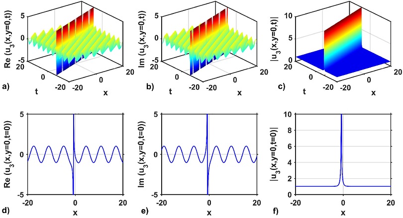
Figure 1 3D structures of the solution u3 (x, y = 0, t): a) real part, b) imaginary part, c) modulus, and d)-f): 2D line plots of a)-c) at t = 0, respectively, for selecting the free parameters values as a = 1.01, b = 1, σ = 1, κ = 1, p = 1, q = -3.5, M = 1.5, P = 1.3, η = 0.4, m0 = 1.4 and γ = -1.04.
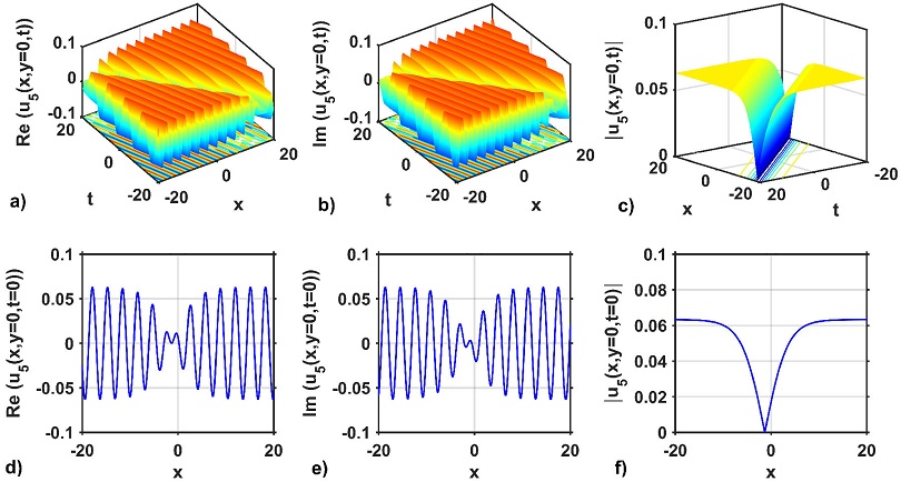
Figure 2 3D structures of the solution u5 (x, y = 0, t): a) real part, b) imaginary part, c) modulus, and d)-f): 2D line plots of a)-c) at t = 0, respectively, for selecting the free parameters values as a = 1.5, b = 2, σ = 0.2, κ = 1, p = 2, q = 1.7, M = 1.5, P = 1.3, η = 0.5, m0 = 2 and γ = -0.02.
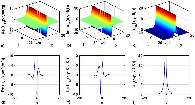
Figure 3 3D structures of the solution u15(x, y = 0, t): a) real part, b) imaginary part, c) modulus, and d)-f): 2D line plots of a)-c) at t = 0, respectively, for selecting the free parameters values as a = 1, b = 1, σ = 1, κ = 0.01, p = 1, q = 1.5, M = 1, η = 1, m0 = 0 and γ = -0.1.
The modulus of the optical solution u15(x, y = 0, t) also demonstrate the anti-bell soliton solution, which is depicted in Fig. 2c). As shown in Fig. 2f), the 2D graph at t = 0 confirms this type of anti-bell soliton solution. The 3D and 2D wave structures of the solutions obtained from the KMN equation are considered to show the behavior of the solution. In addition, the 3D wave profile is exposed to show the temporal and spatial changes of the obtained optical soliton solution. The 3D wave profile for the real and imaginary parts and modulus of the optical solution u41(x, y = 0, t) are depicted in Figs. 4a)-c) respectively. The optical solution u41(x, y = 0, t) represents the periodic wave solution for the real and imaginary parts, as portrayed in Figs. 4a) and b). On the other hand, the modulus of the above solution represents the kink solution, which is depicted in Fig. 4c). The above mentioned can be confirmed from their 2D cross-sectional views at t = 0, as shown in Figs. 4d)-f).
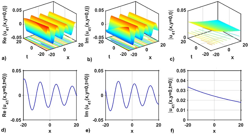
Figure 4 3D structures of the solution u41(x, y = 0, t): a) real part, b) imaginary part, c) modulus, and d)-f): 2D line plots of a)-c) at t = 0, respectively, for selecting the free parameters values as a = 0.01, b = 0.02, σ = 0.59, κ = 0.12, p = 0.52, q = 0.5, M = 2.5, P = 0.1, η = 0.9, m0 = 2.5 and γ = 0.56.
4.2 Impacts of wave dispersion and nonlinearity parameters on soliton pulses
The unified method is applied to the integrable KMN equation to obtain the optical soliton solutions. The obtained solutions involve wave dispersion and nonlinearity terms. The impacts of wave dispersion and nonlinearity parameters on soliton pulses are explained graphically for showing the effectiveness of the unified method.
The impacts of wave dispersion on the attained optical solution |u1(x, y = 0, t)| is shown in Fig. 5 by selecting the free parameters as a = 2.5, b = 0.2, κ = 0.01, p = 2.5, q = -2.5, M = 0.02, P = 0.021, η = 1, m0 = 1, and Y = -0.25 For choosing the dispersion parametric values σ = 0.1, 0.3, 0.5, 0.7, and 0.9, the soliton profiles of the solution |u1(x, y = 0, t)| are presented in Figs. 5a)-e), respectively. The wave profile can change for different σ values. The cross-sectional variation at t = 1of the soliton profiles along the x-axis is displayed in Fig. 5f). In Fig. 5f), it can be seen that the soliton profiles along the x-axis are changed for all values of dispersion, σ = 0.1, 0.3, 0.5, 0.7, and 0.9.
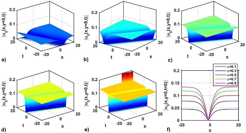
Figure 5 Impacts on wave dispersion on the solution |u1 (x, y = 0, t)|: a)-e) for σ = 0.1, 0.3, 0.5, 0.7 and 0.9, respectively, with a = 2.5, b = 0.2, κ = 0.01, p = 2.5, q = -2.5, M = 0.02, P = 0.021, η = 1, m0 = 1, γ = -0.25 and f) the variation of the soliton profiles at t = 1 of a)-e) along with x-axis.
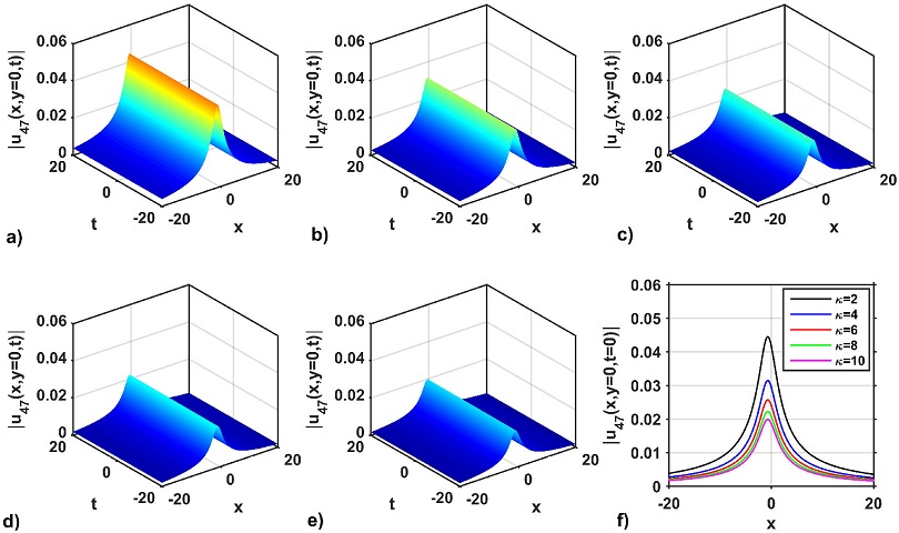
The amplitude of the wave profiles is increased when the value of the dispersion parameter σ decreases. Again, the 3D and 2D shapes of the wave profile of the optical solution |u25 (x, y = 0, t)| is depicted in Figs. 6a)-f). As seen in Figs. 6a)-e), the 3D wave structure represents the periodic wave solution for the dispersion values σ = 0.06, 0.09, 0.12, 0.15, and 0.18, respectively, with the free parameters as a = 1.2, b = 1, κ = 1, p = 1, q = 1, M = 0.07, P = 0.03, η = 1.5, m0 = 4.6, Y = 1.5. Figure 6f) represents the 2D combined graphs of the solution |u25 (x, y = 0, t)| for selecting the distinct dispersion values σ = 0.06, 0.09, 0.12, 0.15, and 0.18. In this case, it can be observed from Fig. 6f) that the amplitude of the soliton increases as the values of σ increase. It is also seen from Fig. 6f) that the signal of the wave profile solution is moved to upward positive values. However, the periods of the solitons are almost the same. Furthermore, the 3D and 2D wave profiles of the solution |u47 (x, y = 0, t)| are presented in Figs. 7a)-f). The 3D wave structures of the solution |u47 (x, y = 0, t)| is presented in Figs. 7a)-e) for distinct dispersion values σ = 0.01, 0.05, 0.10, 0.15 and 0.2, respectively, to select the free parameter values as a = 0.15, b = 0.1, κ = 1, p = 1, q = -1, M = 1.1, P = 0.1, η = 0.1, m0 = 1.5, Y = 0.03. The solution of |u47 (x, y = 0, t)| represents the bell-shaped profiles. To confirm such shapes and characteristics of Figs. 7a)-e), the line variation of the profiles at t = 1 is shown in Fig. 7f). It is seen from the Fig. 7f) that the amplitude of the wave profiles of the solution |u47(x, y = 0, t = 1)| increases with the increase of the values σ. On the other hand, the impact of the nonlinearity parameter of solutions |u45 (x, y, t)| and |u47 (x, y, t)| are shown in Figs. 8 and 9, respectively. It is palpable from Figs. 8a)-e) that the intensities of the periodic wave profile decrease due to the increase of the nonlinearity parameters κ = 1, 1.2, 1.4, 1.6 and 1.8, respectively. To justify such shapes and characteristics of Figs. 8a)-e), the line variation of that profiles at t = 1 is presented in Fig. 8f). The same behaviors are also found and displayed for the bright shape soliton profiles, which are presented in Figs. 9a)-f). From the above mentioned discussion, it is reasonable to mention from the graphical outputs that the wave dispersion (σ) and nonlinearity (κ) parameters of the model can play a notable role in increasing and decreasing the wave profile intensity for displaying the new wave characteristics. Therefore, it is also confirmed from the above mentioned discussion that the soliton profile remains unchanged owing to the balance of the wave dispersion and nonlinearity impacts of the model. It is worth mentioning that no experimental results have been produced and compared with our produced results due to the lack of experimental equipment in our laboratory. Therefore, the choice of wave dispersion and nonlinearity parameter values of the optical solutions are predicted. For this reason, it was quite difficult to sort out the types of fiber or laser and their wavelength, which are the main limitations of our study.
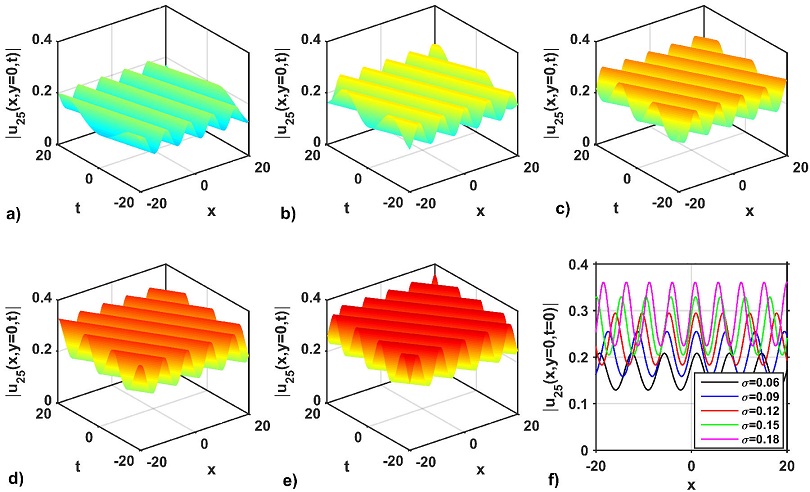
Figure 6 Impacts on wave dispersion on the solution |u25 (x, y = 0, t)|: a)-e) for σ = 0.06, 0.09, 0.12, 0.15 and 0.18, respectively, with a = 1.2, b = 1, κ = 1, p = 1, q = 1, M = 0.07, P = 0.03, η = 1.5, m0 = 4.6, γ = 1.5 and f) the variation of the soliton profiles at t = 1 of a)-e) along with x-axis.
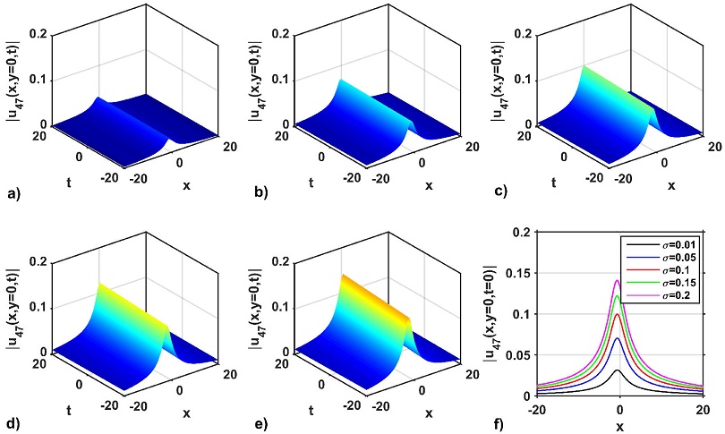
Figure 7 Impacts on wave dispersion on the solution |u47 (x, y = 0, t)|: (a)-(e) for σ = 0.01, 0.05, 0.10, 0.15 and 0.2, respectively, with a = 0.15, b = 0.1, κ = 1, p = 1, q = -1, M = 1.1, P = 0.1, η = 0.1, m0 = 1.5, γ = 0.03 and (f) the variation of the soliton profiles at t = 1 of (a)-(e) along with x-axis.
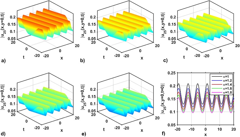
Figure 8 Impacts on nonlinearity of the solution |u25 (x, y = 0, t)|: a)-e) for κ = 1, 1.2, 1.4, 1.6 and 1.8, respectively, with a = 0.15, b = 0.1, σ = 0.06, p = 1, q = -1, M = 1.1, P = 0.1, η = 0.1, m0 = 1.5, γ = 0.03 and f) the variation of the soliton profiles at t = 1 of a)-e) along with x-axis.
5 Conclusion
Implementing the unified method to the KMN equation, we have received some new optical solutions representing the dark, bright, periodic, bell, kink, and singular solitons. We have displayed some 2D and 3D graphs of some received representative solutions including bright, dark, singular, and periodic wave solutions by selecting appropriate values of the free parameters to understand the impacts of wave dispersion and nonlinearity parameters of the KMN equation. For the bright, dark, and periodic wave solitons, it is seen that the wave amplitude increases when the wave dispersion (σ) increases. On the other hand, the wave amplitudes of the bright soliton and periodic wave decrease due to the increase in the nonlinearity parameter (κ). Thus, the amplitude of the soliton profile remains unchanged due to the balance of the wave dispersion and nonlinearity impacts of the model. The validity for the resulting outcomes was performed by substituting the attained solutions back into the equation of our choice through the use of Maple 17. Thus, the complete study approves that the executed method is a powerful tool for producing a variety of optical soliton solutions to NLEEs arising in optical fibers, and optical engineering. The outcomes obtained in this study may illuminate the researchers for further studies to understand the unseen behaviors of soliton profiles in the field of fiber optics and optical communications.

