


 nova página do texto(beta)
 Inglês (pdf)
 Artigo em XML
 Referências do artigo
 Enviar este artigo por email
 Citado por SciELO
  Similares em
SciELO
Similares em
SciELO 
 Permalink
1. Introduction
About 15% of world’s population has medical disabilities of some kind. That is approximately around one billion people worldwide1. As an example, one out of 20,000 people is diagnosed with Amyotrophic Lateral Sclerosis (ALS), a neuro-motor disability that degenerates motor neurons reducing their ability to communicate with muscles2. There are 8 million people with motor disabilities or motor limitations in Mexico3. Of those, 2.6 million have motor disabilities, of which 38.5% are due to some comorbidity4. Motor disability is one of the subtypes of disabilities that most limit the quality of life of those affected by them.
A brain-machine interface (BMI) or brain-computer interface (BCI) is a communication system that allows direct interaction between an electronic device and brain activity. It could be designed through different technologies, such as EEG, MEG, ECoG, EMG, etc.,5,6. People with stroke, cerebral palsy, muscular dystrophy, spinal cord damage, amputated limbs, and mostly with any motor disability, could be physically or socially rehabilitated using some BMI. This would allow them to control a robotic prosthesis, electric wheelchair, computer cursors, or simply communicate through a binary system interpretable as “yes" or “no" responses. In less severe cases such as hemiparesis for example, even proper detection of imagined movements (or motor imagery, MI) could help improve their relationship with the world. This through a reinforcement system that tells patients how well they are imagining a given task. It has been demonstrated that the mere imagination of the realization of their movements during training, produces a significant improvement in the performance of professional athletes7.
BMIs are programmed with algorithms that perform several functions. The main and most relevant are classifiers. Their function is to discriminate data into different classes. A class is the semantic group an event belongs to, defined as loose as one need it to be. For example, an image recognition system that can identify cats and dogs would have 2 classes: Cats and Dogs. And an event is a data point corresponding to one class. On supervised learning, events must be labeled with its corresponding class. On unsupervised learning they do not need to be labeled. There are several and very different classifiers based on their calculations and technology based on machine learning (ML) techniques5,6,8,9. The ones considered for this work are listed as follows.
CSP, Common Spatial Pattern is an algorithm that gets spatial filters from covariance matrices of a given data set. It is considered a feature extraction algorithm because it needs a decision-maker to classify10-13. LDA or Linear Discriminant Analysis projects the data on the hyperplane that maximizes the distance between the means of each class and minimizes the dispersion on the new plane. In the case of scikit learn14, it does so by maximizing the Mahalanobis distance, starting from a Bayes rule. LDA has been used as EEG classifier15-20 and together with CSP21 it has achieved a mean accuracy of 80%.
ANN or Artificial Neural Network, also called multilayer perceptron, is an array of nested perceptrons, capable of learning from examples through iterative corrections on each layer weights. It employs the backpropagation algorithm, which compares the output of each iteration with the expected output and minimizes an error function22. Each perceptron is a mathematical function inspired by how neurons in the brain work. DNN, Deep Neural Networks get their name from the depth of their structure and by having several layers. The intermediate layers between the input and output layers are called the hidden layers. There is no clear definition of how many layers a network needs to be considered deep, however, there is consensus in considering at least 4 layers.23 Deep learning is known for getting good results despite just taking raw data as input, i.e., it automates the feature extraction process. Also, note that the perceptron is a linear machine and the maximum non-linearity it possesses is limited by the activation function. However, by assembling several layers of perceptirons, the net obtains a very important non-linear capacity, since it can model more complex functions and classify data that do not have a linearly separable distribution. It has been widely used for EEG classification24-28.
CNN or Convolutional Neural Networks get their name from the convolutions performed between restricted regions of the neural layer and a kernel, which are a matrix of weights. The result of such convolutions are passed to an activation function. The operation is carried out by taking small steps along the entire layer until all the neurons are covered. It has given very good results on image classification and computer vision29-31. It has also shown good results on MI classification20,32-36. RMDM or Riemannian Minimum Distance to Mean classifier starts from the Minimum Distance to Mean (MDM) algorithm, which compares events in an euclidean space through the distance between them. The Euclidean distance is defined as δE(a,b) = |a - b| where a and b are points in the space. Suppose a simple case with 2 classes, the “rest" class equal to 0 and a class C. Let σ0 be the mean-variance of the events labeled as 0, σC the mean-variance of the events labeled as C, σk the variance of the event k, and δ(⋅,⋅) the distance function. MDM classifiers will simply compare if δ(σC, σk) > δ(σ0, σk) → k belongs to class C. If the opposite is true k is assigned to class 0. RMDM compare instead the Riemannian distance, or geodesic, from an event C to the Riemannian or Cartan mean, representing a kind of center of mass, in a differentiable manifold made up from the set S(++) of N(N covariance matrices, where N is the dimension of the feature space37,38.
Finally, there are different approaches to train a classifier. One is to teach them with part of the data from the volunteers under study. This is called ‘per-subject training’. Other option is to use all the data from all the volunteers for training. That is named ‘global training’. Care must be taken to avoid overfitting in the second scenario. That is, using the same data used to learn to perform predictions on the data. That forces the resulting model to fit the shape of that dataset exclusively and results will always be very “successful". But the truth is, that the rate of success will only be achieved in that data set used to develop the classifier, and it will not be successful at all with other data sets, making results un-reproducible.
Nowadays, clinical BMIs present limited classification capabilities, usually limited to 2 or 3 classes. There have been several studies looking into improving classification accuracy on multiclass cases or improving the computing time required to detect MI in real-time. But clearly further work is needed yet to improve BMI’s ease of use. The aim of this work was to build a low-cost, portable, easy-to-use and reliable EEG-MI based BMI; comparing the classifiers mentioned above to find the one that best satisfies such conditions. Their use would allow people with disabilities to improve their life quality. Different classifiers developed with other technologies and the ones developed here are compared latter in the discussion. Finally, and only for results presented in this paper, parameters such as: accuracy, computing time, kind of training, EEG channels number and sampling frequencies, were considered and a recommendation on which algorithms produced the best results made.
2. Materials and methods
For this project, own laboratory data together with public EEG data were used to compare the efficacy of the implemented algorithms.
2.1. Public Data
The public EEG Motor Movement/Imagery PhysioNet Dataset39 was used. It is available at https://physion et.org/content/eegmmidb/1.0.0/.
2.1.1. Volunteers
Data from 109 subjects in the dataset were available, but only data from 92 subjects was used. Data from volunteers: 14, 34, 37, 41, 51, 64, 69, 72, 73, 74, 76, 88, 92, 100, 102, 104, 109 were excluded since those had fewer events or trimmed events. This was decided to keep the number of events per subject as homogeneous as possible. Data were recorded at the Wadsworth Center BCI Research and Development Program40. No more information about the volunteers was provided by PhysioNet website.
2.1.2. Data acquisition
Each subject in this database underwent 14 runs (actions) which could either be Baseline measurements or Tasks:
1. Baseline, eyes open, 2. Baseline, eyes closed, 3.Task 1 (open and close left or right fist), 4. Task 2 (imagine opening and closing left or right fist), 5. Task 3 (open and close both fists or both feet), 6. Task 4 (imagine opening and closing both fists or both feet), 7. Task 1, 8. Task 2, 9. Task 3, 10. Task 4, 11. Task 1, 12. Task 2, 13. Task 3, Task 4.
“Baseline" (BL) EEG recording are those in which a subject is not performing any special activity: physical or mental. The subject is simply asked to remain relaxed and seated in a comfortable position. For simplicity, this study only used baseline 1 information (with eyes opened).
The recording of the baseline measurements lasted 1 minute each, and 2 minutes for each task. On each task, the subject was asked to perform 5 or 6 times each of the 2 possible moves. Either imagination or the real moves. For example, in Task 1, the subject was asked on 5 occasions to open and close his right fist for 6 seconds; and on 6 times was asked to open and close his left fist for 6 seconds. Each of this 11 times was a 6 second event from Task 1.
Each Task lasted for 2 minutes, and each Baseline run for 1 minute. 3 s events were considered to mimic the data acquisition structure from our lab data (see explanation in the lab data acquisition in following sections). Therefore, Baseline runs were formed by 20 events and Task runs were formed by 45 events. As PhysioNet’s dataset sampling frequency was 160 Hz, the first 3 s of each run corresponded to 480 data points (events). For simplicity, calculations from the authors just used information from these initial 3 s for each run. Also, and for simplicity, in this work authors just used information from Baseline 1, and runs from Task 2 (runs number 4, 8 and 12) which corresponded to imaging of opening and closing left or right fists. Each of these 6-second intervals when the volunteer imagined or executed a move, was considered an event. So, for each of the 92 subjects there were 45 events of each task. Again, for simplicity, only the data from Task 2 (actions number 4, 8, and 12) were considered, which corresponded to imaging opening and closing the left or the right fist. And the events were trimmed, taking only the first 3 seconds of each. The latter to match them up with the length of the events in the Lab Data (see the details of laboratory data in the following sections). Likewise, the entire Baseline recording was divided into 3-second sections. So, 20 baseline events per subject were obtained.
Ideally, when training a machine learning model, the number of events per class should be similar. As data in Baseline and Task runs were imbalanced in favor of Task runs, a data augmentation procedure was used. ‘New’ Baseline events were generated by joining the final half of an event with the initial half of the contiguous one. Thus, instead of having only 20 events per subject, we now had 39 events per subject. This produced a total of 3588 baseline events (considering the 92 subjects), and 4140 Task 2 events, of which 2086 corresponded to the left fist and 2054 to the right fist.
2.1.3. EEG
A 64 channel EEG (unknown brand) was used, with a sampling frequency of 160 Hz. Electrodes were placed according to the international 10-10 system, excluding: Nz, F9, F10, FT9, FT10, A1, A2, TP9, TP10, P9, and P10. Data were then recorded using the BCI2000 system (http://www.bci2000.org), on a PC with “1.4-GHz Athlon processor, 256 Mb RAM, IDE I/O subsystem, and Data Translation DT3003 data acquisition board, running Windows 2000"41. Time sequences were provided in edf files.
2.2. Lab Data
This dataset was generated in our laboratory, at the Facultad de Ciencias Físico Matemáticas, Benemérita Universidad Autónoma de Puebla, Mexico.
2.2.1. Volunteers
EEG data were obtained from a sample of 30 right-handed male volunteers without a clinical diagnose of psychiatric, psychological, or neurological pathologies. Ages ranged between 18 and 31 years old. They were students and faculty members of the physics department. Everyone claimed to have slept more than 6 hours the night before experimentation and were not under the effect of psychoactive drugs or under any kind of medical treatment.
2.2.2. Data acquisition
This protocol was mainly based on the work of Brunner et al.42, Lee and Choi43 and Wu et al.44. Experimental runs were made in a well-lit laboratory, with little noise and no noteworthy odors, seeking to reduce external stimuli that could affect the experiment. Volunteers were asked to sit so that they were comfortable one meter away from a screen showing a sequence of images related to a task, (presentation in Microsoft PowerPoint (http://www.office.com). The screen was the one of a laptop with a LED display, 1920(1080 resolution, and 60 Hz frequency. The protocol is presented here:
2.2.3. Runs
First, a 30 second run was made to record eye-open baselines. A complete cycle was defined as a complete set of rest - movement - rest - imagination. I.e., cross - solid arrow - cross - faint arrow. All this with a total duration of 12 seconds as shown in Fig. 1. A uniform pseudorandom succession was generated with Python NumPy of 48 cycles, 24 for each side of the body, presented to volunteers in 3 blocks of 16 cycles each. This protocol generated a total of 10 minutes and 6 seconds of EEG recording per subject. Finally, a total of 300 baseline events and 720 events of each motor imagery side were used. To handle the data imbalance, a data augmentation technique was applied to the baseline events. A new event from the last and first half of contiguous events was made. This allowed authors to get up to 590 baseline events, closer to the 720 of each of the other classes.

2.2.4. EEG
Data were acquired with an Emotiv EPOC+ headband EEG (https://www.emotiv.com/epoc/). Sampling frequency of 128 Hz, 14 electrodes standardized according to the international 10-20 system (AF3, F7, F3, FC5, T7, P7, O1, O2, P8, T8, FC6, F4, F8, AF4). It had built-in notch filters of 50 and 60 Hz. EmotivPRO v1.8.1 commercial software was used as a PC-Emotiv interface connected via built-in Bluetooth.
2.3. BMI Architectures
In this study, the accuracy of each classification model was compared on 4 comparison groups: left MI/right MI (LMIvsRMI), left MI/baseline (LMIvsBL), right MI/baseline (RMIvsBL), and the 3-class left MI/right MI/baseline (LMIvsRMIvsBL). For both, training and validation, each event was 3 seconds long, corresponding to 384 EEG samples in the lab data case.
Both, global and per-subject training, were performed with each of the BMI’s to compare the efficacy of each classifier with big and small data and with their generalization capability.
2.3.1 Programming hardware and software
The different machine learning models were run on a commercial PC, with 32 GB RAM, 3.4 GHz Intel Core i7 - 6700 CPU, NVIDIA GeForce GTX 1070 GPU, running Windows 10. BMIÂs were coded in Python (https://www.python.org/) using the Keras framework (https://keras.io/), sklearn (https://scikit-learn.org/), and pyRiemann libraries (https://pyriemann.readthedocs.io).
2.3.2. CSP + LDA
Raw data were set in an ExNxT matrix, re-referenced to the common average reference (CAR), and then balanced and normalized. Following this, data was band-passed and filtered by a Butterworth 6-order filter with an 8 to 30 Hz window. CSP was computed using the MNE package (https://mne.tools/), with the Ledoit-Wolf method for covariances estimation. 6 CSP were used as feature vector input of each LDA classifier.
2.3.3. DNN
Data were first centered between [-1,1] by the sklearn’s maxAbsScaler function. A fully connected deep neural network (DNN) with 9 hidden layers was used. The kernel initializer was the same along the net: Random Uniform between (-0.05, 0.05), using 42 as seed. Leaky ReLU with alpha=0.3 was used as the activation function in the inner layers, to prevent the death of neurons with negative values as output, conserving a small gradient; and Softmax was placed in the output layer because it could be used with any number of classes. Nesterov-accelerated Adaptive Moment Estimation (Nadam) was used as the optimizer, because a rapid convergence method was needed to not extend much the training time45, with learning rates between 1(10-6 and 1(10-9, and cross-entropy as the loss function. 30% of dropout on each layer was considered. The training was done in about 30 to 100 epochs, empirically tuned taking care of both underfitting and overfitting by comparing the training accuracy with the validation accuracy.
2.3.4. CNN
A convolutional neural network (CNN) with the architecture proposed in Dose et al.34 was used for this BMI. It consisted of two convolutional layers of 40 neurons each. The first one included no padding, with a 30(1 kernel. The second included a zero padding with a 1(64 kernel. In both cases, the default (1,1) stride was used. The next step was a 15(1 max pooling with zero padding, then data was flattened. The next layer was a fully connected layer with 80 neurons. Finally, the output layer contained 2 neurons. However, the kernel sizes of the layers were adapted when training the lab data as follows: 24x1, 1x14, and 4x1 respectively. The kernel initializer and the activation functions maintained the same conditions as with DNN.
The intuition behind this array was based on letting the CNN do the feature extraction. The first convolutional layer was expected to work as a spatial filter among the channels. Whereas the second one, made a temporal filter among the samples. So, its input were the raw data in matrix form of NxT, in which N was the number of electrodes and T was the samples of each event. Then, “filtered" data were flattened and passed through an additional neuron layer for the main classification. The structure is sketched in fig. 2.
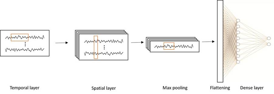
Figure 2 CNN architecture. The CNN BMI consisted of one temporal layer in which a horizontal kernel (box in red) extracted the time domain features from the time series of each channel. Then a spatial layer in which a vertical kernel extracted the features related to the position of the channels in a time window. After this, Max pooling was performed to summarize the previous learning, and finally data were flattened and passed through a fully connected layer.
2.3.5. RMDM
This classifier was based on the work of Congedo et al.38. Events were bandpass filtered by a Butterworth 6-order filter with an 8 to 30 Hz window. Filtered data resulted in an ExNxT matrix, in which E was the number of events, N was the number of channels and T was the number of samples. This matrix was the input to the RMDM. The Riemannian mean of each class and the distance from every event to the means, were computed with the help of the pyRiemann library. Then, a 5-fold cross-validation of the scores was performed.
3. Results
A summary of the mean accuracy obtained with the different classifiers is presented in Table I. It presents results separated by algorithms, public or lab data and wither global or each-subject training was used. Each row represents a classification group (LMIvsRMI, LMIvsBL, RMIvsBL, or LMIvsRMIvsBL) using a specific algorithm.
Table I Results summary. Summary of global and per-subject results with the 4 algorithms on lab and public data. The best result by row is highlighted in bold.
| Lab data | Public data | ||||
|---|---|---|---|---|---|
| Algorithm | Classes | Mean Acc per subject (%) | Mean Acc per Global (%) | Mean Acc per subject (%) | Mean Acc per Global (%) |
| CSP+LDA | LMI/RMI | 48.1 ± 6.7 | 49.7 ± 3 | 51.4 ± 8.2 | 49.8 ± 1.7 |
| LMI/BL | 99.7 ± 1.3 | 100 | 95.1 ± 14.3 | 97.9 ± 0.3 | |
| RMI/BL | 99.8 ± 1.2 | 99.9 ± 0.2 | 95.1 ± 13.7 | 98.1 ± 0.3 | |
| LMI/RMI/BL | 61.6 ± 4.5 | 64.1 ± 1.6 | 69.1 ± 11.1 | 73.4 ± 1.3 | |
| DNN | LMI/RMI | 65.6 ± 3.5 | 50.2 ± 1.3 | 70.2 ± 4.2 | 71.4 ± 1.2 |
| LMI/BL | 68.8 ± 4.5 | 56.5 ± 1.8 | 72.5 ± 3.7 | 86.4 ± 0.4 | |
| RMI/BL | 81.5 ± 2.7 | 56.6 ± 1.7 | 73 ± 12.1 | 86.9 ± 0.4 | |
| LMI/RMI/BL | 54.5 ± 4.1 | 29.3 ± 1.6 | 54.2 ± 3.1 | 73.6 ± 1.3 | |
| CNN | LMI/RMI | 50.6 ± 2.9 | 50.1 ± 0.2 | 52.3 ± 6.5 | 59.5 ± 0.4 |
| LMI/BL | 56.8 ± 8.8 | 56.6 ± 1.7 | 59.5 ± 11.7 | 98.4 ± 0.2 | |
| RMI/BL | 60.1 ± 13.5 | 43.4 ± 1.7 | 61 ± 10.7 | 98.3 ± 0.5 | |
| LMI/RMI/BL | 33.7 ± 3.9 | 56.6 ± 1.7 | 44.2 ± 9.7 | 74.7 ± 0.3 | |
| RMDM | LMI/RMI | 51.1 ± 8.1 | 50.7 ± 2.4 | 53.8 ± 13.4 | 57.9 ± 1.9 |
| LMI/BL | 100 | 100 | 97.1 ± 11.2 | 99.9 ± 0.1 | |
| RMI/BL | 100 | 99.9 ± 0.2 | 97 ± 11.4 | 99.9 ± 0.1 | |
| LMI/RMI/BL | 63.3 ± 6.2 | 63.6 ± 4 | 72 ± 13.1 | 77.5 ± 0.9 | |
Figure 3 Presents a graphical representation of accuracy vs. classes. This was done to assess the relationship between lab and public datasets. It is presented in the same format as Table I, subdivided through the different algorithms, to be able to see which was the best classifier on each case.

Figure 3 Accuracy vs. classes. The vertical axis presents the accuracy (%). There are 4 blocks corresponding to the 4 algorithms used, and 2 sub-blocks corresponding to the 2 datasets used, i.e., the public or lab data. Each color represents a classification group: LMI is for Left Motor Imagery, RMI for Right Motor Imagery, and BL for Baseline. The black dots represent the outliers beyond the quartiles considered on the boxplot.
The comparison between results when performing global and/or per-subject training is presented in Fig. 4.

4. Discussion and conclusions
The main findings of this work were that the mean accuracy for each classifier was 78%, 66%, 60% and 80%, for CSP, DNN, CNN and RMDM, respectively. The best results were obtained in baseline vs MI. With global-training public data, an accuracy between 86.4% and 99.9% was achieved. With global-training lab data, the accuracy was above 99% just for the CSP and RMDM cases. For lab data, the classification/prediction computing times per event were 8.3 ms, 18.1 ms, 62 ms and 9.9 ms, for CSP, DNN, CNN and RMDM, respectively, which shows the viability of using these algorithms in a real-time BMI.
All the four algorithms had some trouble discerning between left and right motor imagery, but almost all had good performances classifying motor imagery versus baseline, regardless of laterality, in both public and lab data. It is important to note that, for the four algorithms, the per-subject-training mean error was about 10% higher than the global training error. This was due to the high variance in the results among volunteers; for just one subject the accuracy was 20%, while that of the rest remained close to 99%. This amplitude is blurred in global training, where internally the classifier considers these differences.
In addition, if it the data imbalance is only considered, lab data were expected to have at least 50% accuracy on left vs right MI, 44.2% on both left MI vs baseline and right MI vs baseline, and 28.4% on 3-class classification. On the other hand, for public data, the expectations were 49.6%, 36.8%, 36.4%, and 26.6%, respectively. Of course, for practical reasons, the actual expectation should be above 50% for these classifiers to be useful.
4.1. Computing time
Table II presents the average computing time per event. The training time depended heavily on the hardware used and the GPU used here was an average commercial element. Considering about 5000 events on a 2-class problem, it took about 45 minutes for CNN to be ready, which was the longest. The fastest algorithm was CSP, taking less than 5 minutes to be ready. However, the most important part was the prediction time to identify if it could be used in an actual real-time BMI. When considering the lab data, with a sampling frequency of 128 Hz (every 8 ms a sample was taken). If each event were 3000 ms long, even the slowest algorithm, CNN, could have made 48 predictions in the time of an event. At most, it could miss 7 samples out of 384 from an event. The fastest classifier, CSP, could make 361 predictions. DNN 165, and RMDM 303 predictions. So, these results show that any of the BMI’s presented here, were viable for clinical use within a 3 s window.
Table II Computing time. Average computing time per event and by algorithm on training and prediction.
| Average training time/event (ms) | Average classification time/event (ms) | |||
|---|---|---|---|---|
| Algorithm | Lab data | Public data | Lab data | Public data |
| CSP+LDA | 14.2 ± 0.3 | 55.3 ± 1.2 | 8.3 ± 0.2 | 34.4 ± 0.8 |
| DNN | 20.7 ± 0.7 | 212.5 ± 2.5 | 18.1 ± 1.2 | 117.8 ± 7.3 |
| CNN | 85.1 ± 1.3 | 524.1 ± 3.2 | 62 ± 3.6 | 373.2 ± 11.7 |
| RMDM | 17.5 ± 0.3 | 98.5 ± 0.7 | 9.9 ± 0.4 | 46.2 ± 1.2 |
4.2. Classifiers evaluation
The highest classification accuracy was obtained by RMDM in both public and lab data. Particularly, on MI vs. Baseline, classification reached values above 97%. For lab-data per-subject RMI vs BL achieved a 100% accuracy, this means it was able to detect MI on each subject for every event. CSP performed closely with 99.8% ± 1.2% in the same category, and with more than 95% on MI vs BL. Of course, considering they took the data from only 30 people, they may be overfitted and further work is needed to test them with new data. Unfortunately, on the left MI vs. right MI classification, they were not able to make a discriminant prediction. Probability values were so low that they were not better than just guessing. Only in the public global case, RMDM got an acceptable 57.9% ± 1.9% at best. This could imply a need for more data to improve the results. However, as stated before, the similitude between results on lab and public data shows the algorithm’s consistency while working with both few and big data. Even in the multiclass case, both CSP and RMDM did well with results between 61.6% ± 4.5% and 77.5% ± 0.9%. DNN and CNN gave very similar and conservative results. However, they produced better results classifying LMI vs RMI than the previous 2 classifiers. Although for lab data they obtained mainly around 50% accuracy, in public data they showed an improvement up to 71.4% ± 1.2%. Specially DNN, consistent with the suitability of the DL for large amounts of data, with the advantage that it practically did not require preprocessing and could handle raw data. Figure 2-4 showed that both had a significant difference for global training results between public and lab data, but in the training per subject, there was no substantial difference. This could be due to the fact that the amount of data from a single user was not so extensive, so that it did not exploit the benefits of deep neural networks. Likewise, both obtained satisfactory results for MI vs baseline classification, and CNN gave 98.4% ± 0.2% and 98.3% ± 0.5% accuracies in the global public case.
4.3. Comparison results with State-of-the-art results
In the literature, MI classifiers present accuracies above 60% ± 1.8%, based on16-21,25-28,32-36,43,46-55. Most of them took data from 2 to 10 subjects and used 64 to 128 EEG channels, as shown in Figure 5. For studies using Emotiv as an EEG, accuracy has been found to be even higher (above 80% ± 10.6%), such as in21,25,46-48. However, the average accuracy of the whole study in our case was about 70%. Nevertheless, if just public data were the considered by us, a decision most of the literature experiments have followed, the accuracy would be circa 81%.

Figure 5 Motor imagery classifiers vs. accuracy. This is a representation of the mean accuracy obtained by MI classifiers in the literature. The data were taken from all the cited studies on this work. The last blue bar represents the average accuracy obtained in this study considering the 4 algorithms, the 4 classification groups, as well as global training. Source: Prepared by the authors based on16-21,25-28,32-36,43,46-55.
For CSP, the literature sets the accuracy bar around 80% ± 7.7%11,21,46,47,52, and for LDA around 72% ± 5.4%16-21, as shown in Figs. 5 and 6. Here, the accuracy improved on the MI vs Baseline case to results higher than 97.9% ± 0.3%. It is interesting to note that the accuracy threshold on lab data was 99.7% ± 1.3%, practically 2 points more than the one on public data. This could raise some concerns about overfitting. But the consistency on getting high accuracies in both cases confirmed the utility of this algorithm and its independence on high amount of data to perform well.
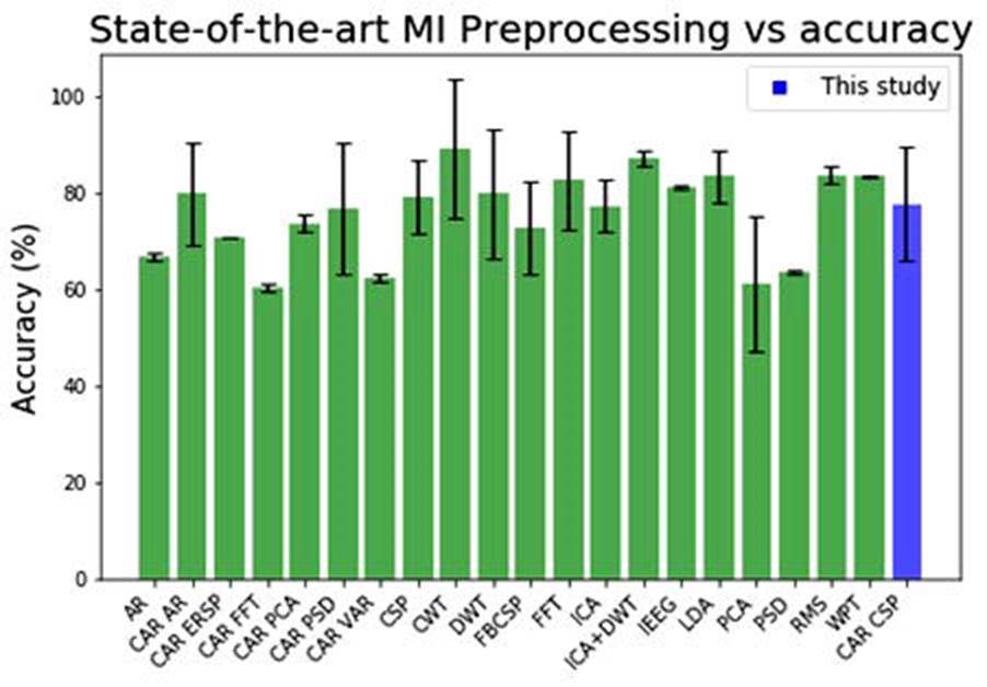
Figure 6 MI preprocessing algorithm vs. accuracy. Here preprocessing used in state-of-the-art literature results is compared with the mean accuracy obtained independently of the implemented classifier. Source: Prepared by the authors based on16-21,25-28,32-36,43,46-55.
Turning to the subject of neural networks, the literature presents a boom of studies implementing this technology, and surprisingly, obtaining good results maintaining around 80% accuracy even in the classification of 2 types of MI, and around 60% for the multiclass case.20,25-28,32-36,43,44,48,51 Considering only the case of public data and global training, to make a fairer comparison, in this work an average accuracy of 81% was achieved.
4.4. Limitations
Since CSP looks to maximize the variance among classes, it could be concluded that there was not sufficiently distinctive variability among MI signals, or at least not distinct enough to be linearly separated by LDA. This could be attributed to the leak of MI-sensitive EEG channels, such as C3 and C4 on Emotiv. But it was immediately refuted by contrasting with the PhysioNet results, which EEG which did include electrodes on the central zone of the scalp, even C1, C2, C5, and C6.
The similarity in the results of CSP and RMDM can be explained considering that both methods were based on finding the covariance matrices of each class. To achieve an improvement, it was necessary to guarantee high variability between classes. This could be done through the method of obtaining the covariance matrices, or increasing the spatial resolution of the equipment, or using a different EEG referencing according to the spatial relationship of the classes. One could also think of separating the electrodes, using only those on the right side of the head in the left MI tasks and vice versa. But the challenge would then be to translate the data so that the interface was able to include this separation in the implementation.
Nowadays understanding about the inner workings of neural networks, does not yet allow us to precisely define what do each filter and/or kernel imply. When it came to image recognition, there was a linear analogy to turn to, considering such weights as filters that detected angles and shapes. But when it came down to EEG signals, there was no similar analogy to turn to. In a certain way, neural networks were seen as black boxes whose fine-tuning required an artisanal process, modifying the hyperparameters until the architecture that generated a correct model was achieved. With little or no preprocessing, to expect satisfactory performance on EEG using neural networks large amounts of data was required.
4.5. Future work
In general, global training produced higher accuracies. This showed a viable path for the development of DL-based BMIs. That is, doing global training to initialize the classifier network, but then calibrating it through transfer learning with data from the particular subject to adapt the interface. Subsampling public data to match it with the lab data shape (14 channels and fs=128 Hz) could be done, and train then the algorithm with the sum of both datasets as input. The use of specially designed EEG for BMI with few electrodes (about 4) in strategic regions that guarantee the right spatial resolution for MI tasks should be explored. The most promising results were obtained with RMDM and CSP so when used combined, taking CSP as the covariance matrices for RMDM could rise the accuracy, and would take advantage of the best features of each algorithm. But more data is needed, ideally taken from different subjects, to verify and solve the overfitting on these classifiers. And more research is needed to reduce the events’ time and take the BMI closer to a real-time solution.
4.6. Conclusions
The overall mean accuracy was better for the case with public data and global training. But when considering individual results, the training per subject gave promising results in most cases, although the high variability between subjects drastically increased the error. Concerning the case of lab data, the results with CNN were not optimal, but with DNN they were acceptable. In contrast, CSP and RMDM results were excellent and demonstrated the feasibility of their implementation for an BMI.
It is important to consider the minimum signal level Emotiv allows is 8400 µV (pp), so its floor noise must be around 8 mV; on the other hand, the floor noise of a typical data acquisition board is about 1 mV. Therefore, the SNR of the PhysioNet data must be higher than Emotiv’s. This has an impact on the feature extraction and, consequently, on the classification of the obtained signals. Finally, here authors presented a portable, affordable, and easy-to-use option, in contrast to clinical equipment. A solution able to detect one MI stimulus accurately, and 2 different MI stimuli with significantly less accuracy though. However, under the 3 s time window per event limitation, it cannot be considered a real-time solution yet.

