


 text new page (beta)
 English (pdf)
 Article in xml format
 Article references
 Send this article by e-mail
 Cited by SciELO
  Similars in
SciELO
Similars in
SciELO 
 Permalink
1. Introduction
The fractional calculus is a generalization of the usual calculus, where derivatives and integrals are defined for arbitrary real numbers. In some phenomena, the fractional operators simulate the phenomena better than ordinary derivatives and normal integrals. Fractional calculus has been widely used in science and engineering1-3; in particular, the study of fractional differential equations such as fractional wave equations have received great deal of attention due to the importance of propagation of electromagnetic waves and vibrating strings4,5. Moreover, the fractional Schrödinger equation has been recently studied in many fields, such as the obstacle problem, phase transitions and anomalous diffusion6-12, etc. Fractional calculus began with Leibniz (1695-1697) and Euler’s speculations (1730); later on, Riemann, Liouville, Grünwald and Letnikov13-16 provided the general definition of fractional derivatives. In 2000, Laskin provided the first application of fractional calculus in quantum mechanics by employing the path integral formulation over Lévy paths and showed that the corresponding equation of motion is indeed the space fractional Schrödinger equation17-20. In Refs.21-24 the authors used the method developed by Laskin to study some new physical applications, its non-locality and the consistency of its solutions. On the other hand, Naber introduced in 2004 the time fractional Schrödinger equation25, where he investigated the wave function of the time fractional Schrödinger equation for free particles and potential wells, and obtained the corresponding wave functions in terms of the Mittag-Leffler function. An overview of quantum mechanics and quantum dynamics with time fractional derivatives can be found in Refs.26,27. In Refs.28,29 the authors solved the space-time fractional Schrödinger equation for free particle and for square potential well using the integral transform approach; moreover, in Ref.30, the Schrödinger equation with Riesz fractional derivative was solved using the scaling transformations. Also, the numerical solution of fractional Schrödinger differential equation with the Dirichlet condition has been investigated in Ref.31. The space-time fractional Schrödinger equation has been obtained by replacing the space and time derivatives of integer order by the derivatives of non-integer order. There are several ways for generalizing an integer-order derivative to the arbitrary case including the Riemann-Liouville and Caputo definitions. In Ref.32, the definitions of the fractional Caputo and Riemann-Liouville derivatives and p-Laplacian operator 𝜙p have been used and the existence of solutions for nonlinear fractional differential has been investigated. Another application of fractional calculus can be found in Ref.33, where the fractional order model HIV/AIDS with the Liouville-Caputo and Atangana-Baleanu-Caputo derivatives has been considered. In this paper, we use the Caputo fractional derivative, defined as13
where for the case α → n, the Caputo derivative becomes an ordinary n-th order derivative of the function ƒ(t).
We consider the space-time fractional Schrödinger equation for the delta potential, then, by imposing a special initial condition we obtain the corresponding wave function by using the joint Laplace and Fourier transforms with respect to time and coordinates, respectively. The Laplace transform of the Caputo derivative is given by13
where
The paper is organized as follows. In 2, we introduce the space-time fractional Schrödinger equation and a special initial condition. In 3, we obtain the wave function corresponding to the imposed initial condition in terms of Fox’s H-function by applying the joint Laplace and Fourier transforms. In 4, the time dependent energy eigenvalues are determined by an asymptotic expansion of Fox’s H-function. The paper ends with the conclusions in 5 and two appendices.
2. The space-time fractional Schrödinger equation for delta potential
The one-dimensional time-dependent Schrödinger equation is given by
where m is the mass of the particle and ℏ is the Planck’s constant; in an analogous way, the one-dimensional space-time fractional Schrödinger equation is written as25
where 0 < ( ≤ 1, 0.5 < β ≤ 1, η = mc2(ℏ/mc2)(. The scaling factors iαη and -(1/2)mc2(ℏ/mc)2β have been added to equalize units on both sides of the equation. It is easy to see that for the special case ( = 1 and β = 1, the space-time fractional Schrödinger equation (4) reduces to the ordinary Schrödinger equation (3). In Ref.22, Eq. (4) was studied for a free particle and for a potential well assuming only the space fractional state; the wave functions and the corresponding eigenvalues were calculated. It was observed that in the case of the free particle, the wave function could be obtained in terms of the Fox’s H-function while for the potential well, the method of separating the variables was used and the solutions of the system were obtained in terms of the space fractional parameter; the some problems were investigated in Ref.25 assuming that only the time fractional case was taken into account. The wave function in the case of the free particle was obtained as the time dependent Mittag-Leffler function multiplied by the spatial function of the free particle, while in the case of the potential well, energy dependent on the time fractional parameter was obtained. Further, in Ref.34, the space fractional Schrödinger equation for single and double Dirac delta potential was considered; the wave functions were determined in terms of the Fox H-function, and the energy eigenvalues were obtained by using the Fourier transform and the Riesz fractional derivative; while the authors assume only the spatial derivative of Schrödinger equation as the Riesz fractional derivative, here, we intend to investigate the Caputo space-time fractional Schrödinger equation for the Dirac delta potential V(x) = -v0 δ(x), that is
We solve the problem analytically by using the joint Laplace and Fourier transforms; to this aim, first we consider the following physical boundary and initial conditions
Choosing an arbitrary function for g(x) one can solve the problem numerically, but in this article we try to choose a specific function for the special case for g(x) so that the problem can be solved analytically. As a result, we shall show that for the special case α = β = 1, the solution of the ordinary Schrödinger equation for Dirac delta potential is obtained. Now to solve the Eq. (5), we apply the joint Laplace transform on the spatial coordinate and the Fourier transform on the time coordinate defined by35
where the symbols for (-) and (∼) are used to denote the Laplace and Fourier transforms, respectively, and k and s are the Fourier and Laplace transform variables.
3. Wave function of one-dimensional space-time fractional Schrödinger equation for the imposed initial condition
By applying the joint Laplace and Fourier transforms to Eq. (5) and using the boundary conditions of Eq. (6), we obtain the following equation
where F=(1/2)mc2(ℏ/mc)2β. The inverse Laplace transform of Eq. (8) gives
In the above calculation, we have used the following formula36
where Eα,β (z) is the Mittag-Leffler function defined as37
Now, we assume the function g(x) as
This choice, as mentioned above, can help us to solve the problem analytically and obtain the analytical solution of the ordinary Schrödinger equation, α = 1 and β = 1. Needless to say, for other choice of the g(x), the analysis is difficult, and perhaps impossible; accordingly, the problem must be solved numerically. Applying the Fourier transform to the relation (12), we get
where
In Appendices A and B, we have reproduced some useful relations about on the Fox’s H-function and its integral according to38; using (B3), (13) is calculated as
Hence, by substituting (21) into (9), we get
Now by calculating the inverse Fourier transform of (16), using the integral containing of two Fox’s H-functions, an taking into account the properties of Fox’s H-function38,39, we get the wave function φ(x,t) in the following form
where β > - (1/2), (α/β) > 0, α + β < 2, ά < (4/3); the definition of the Fox’s H-function of two variables
is given in Eqs. (A.4-A.7). It should be noted here that the acceptable values of α and β above are consistent with the values of α and β, i.e., 0 < α ≤ 1 and 0.5 < β ≤ 1. Before calculating the energy eigenvalues, let us show that the obtained wave function coincides with the wave function of the ordinary Schrödinger equation for the delta function potential; to this aim, we inspect the wave function 𝜙(x, t) in limits of α ( 1, β ( 1, ά ( 1. Using the integral relations of the Fox’s H-function, Eqs. (A.4-A.7), and after some calculations, we arrive at
Then, using the properties of the Gamma function and Fox’s H-function given in Ref.40, the function in (18) is simplified to
Therefore, up to a normalization coefficient A, it is easy to see that the above equation is in agreement with the wave function of the ordinary Schrödinger equation for the delta function potential; choosing
In Fig. 1 we have plotted the probability of the particle presence for some values of β by considering α = ά = 1. Also, the time-dependent effect for different choices of α and β is illustrated in Fig. 2. From Fig. 1 it can be seen that by increasing the parameter β, the probability of the particle presence decreases; the result coincides with Fig.1 in Ref.36 for the non-fractional time derivative of the Schrödinger equation. It can be seen from Fig. 2 that the probability of the particle presence decreases over time; the probability decreases in the central points (x = 0) and increases at the points far from the center. In Fig. 2 the dependence of the probability on time at those points close to the well (x = 0) illustrated for both fractional modes, space and time. Also, it is seen that by decreasing the fractional state (α ≈ 1 and β ≈ 1), the dependence of the probability on time disappears.
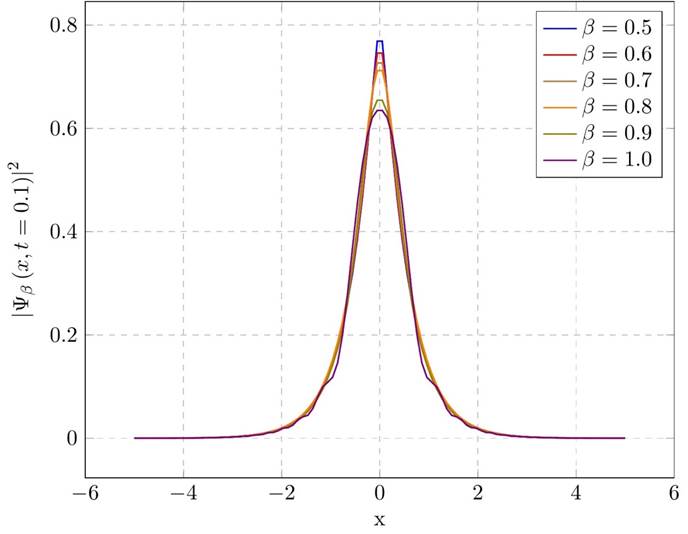
Figure 1 Plot of Eq. (17) as a function of x for α = 1, ά = 1, t = 0.1 and different values of β; for simplicity, we have chosen m = ℏ = c = λ = 1.
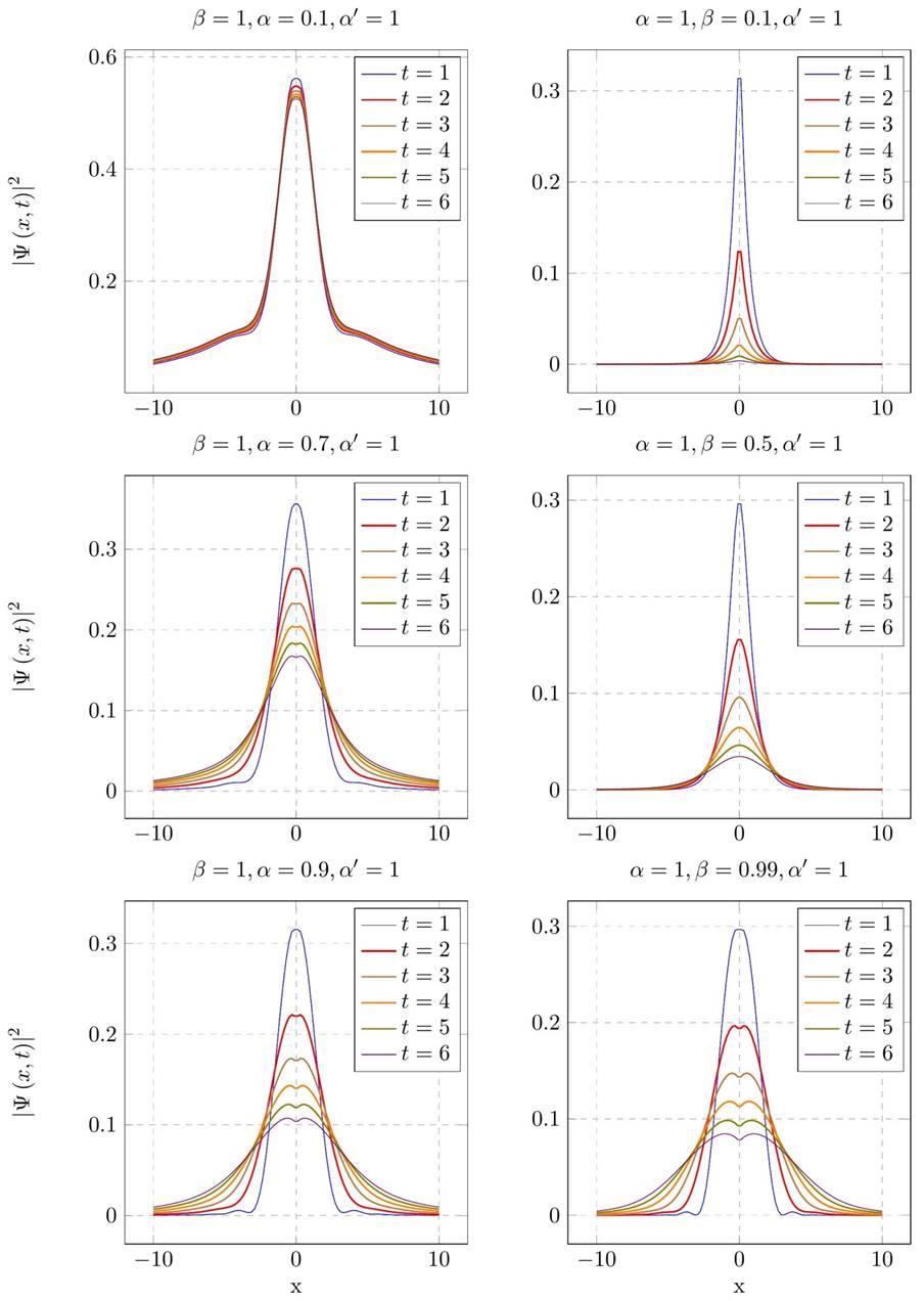
Figure 2 The probability of presence of the particle in dependence on x for different values of time.
In the next section, we shall obtain the energy eigenvalues of the system.
4. The energy eigenvalues of the delta potential for the imposed initial condition
According to Ref.41, for the space-time Schrödinger equation, the energy eigenvalues can be obtained from the equation
First, let us rewrite the wave function (18) in another form of the Fox’s H-function as
Then, using the Caputo fractional derivative of the Fox’s H-function, given in Ref.40, one can calculate the derivative of the first order of the Fox’s H-function of two variables; substituting the obtained result into Eq. (20), we get
To compute the integral, we first express both Fox’s H-functions of two variables in terms of the Mellin-Barnes type integral given in Eqs. (A.4-A.7); then, following the procedure in Ref.35, we obtain
Now, if we use the Mellin transform theorem and substitute s → -η’ -t’ -ξ’ - (½) in Eq. (23), the energy eigenvalue is obtained in terms of the Fox’s H-function of three variables as
which is valid under the following conditions
Thus, it is seen that the energy eigenvalue (24) is time dependent. Also for complex values of the parameters α and β, the energy eigenvalue E may be complex for an unstable system.
Now, let us investigate the energy eigenvalue (24) for the special cases α → 1, β → 1 and ά → 1, that is
In the above relation, we have used identities of the Fox’s H-function of two variables given in Refs.38-40. We also need to use the expansion of the Fox’s H-function at small and large times. For small values of t → 0, using the Fox’s H-function40, the energy is obtained as
5. Conclusions
In this paper, we have studied the Caputo space-time fractional Schrödinger equation for the delta potential. To solve this equation, we have used the joint Laplace transform on the spatial coordinate and the Fourier transform on the time coordinate; then we have obtained an assumption by trial and error, so that the problem can be solved analytically. In other words, assuming that the initial wave function is the Mittag-Leffler function, then the wave function and the energy eigenvalues can be obtained in terms of the Fox’s H-function of two and three variables, respectively. On the other hand, assuming other functions as the initial wave function, solving the corresponding equation is difficult and it must be solved numerically. We also investigated the wave function for particular values of the fractional parameters α → 1 and β → 1 and obtained the results of the standard Schrödinger equation with the delta potential. Moreover, we studied the behavior of the particle presence probability. In Fig. 1, for the case of non-fractional time derivative (α = 1), it was observed that by increasing the spatial fractional parameter (, the probability of the presence decreases which is consistent with the result given in Ref.36. In Fig. 2, we have demonstrated the dependence of probability on the time while it was not the case in the standard Schrödinger equation. We have also shown that the probability of presence is decreased as time increases such that the probability is decreased in the central points (x = 0) and at points farther from the center, the probability of presence is increased. It was also observed that by decreasing the fractional state (α ≈ 1 and β ≈ 1), the dependence of the probability of presence on time disappears. In the end, we investigated the energy eigenvalue for the special cases α → 1, β → 1 and ά = 1; then, we checked the approximate behavior of energy eigenvalue at small and large times. It was observed that while for large times, the energy of the system dissipates, for small times, the energy is in accordance with that of the standard Schrödinger equation for the delta potential.

