1 Introduction

Presently, Altern Current magnetic techniques measure the dynamic magnetic susceptibility of ferrofluids in the absence of external magnetic fields [^1,2,3]. It uses the fact that the Brownian motion of the particles becomes affected by the fluctuations of the macroscopic magnetization created by the Altern currents. Consequently, this technique provides a way to determine several equilibrium properties, including; the particle shape and its diameter [^4,5,6], phase transitions characterization [⁷], the rotational diffusion coefficient of a ferromagnetic particle in a polymer solution [^8,9]. It also allows the measurement of the viscosity of the supporting media [¹]. Ferrofluids are magnetic colloids made of nanometric size ferromagnetic particles dispersed in a solvent. The particles possesses a rigidly attached magnetic moment and perform Brownian relaxation as a single object. The study of the equilibrium dynamics of magnetic fluids have become necessary because their collective behavior is related to diverse technological applications among others in Breast-cancer thermoablation [¹⁰] and hyperthermia health treatments [^11,12,13,14]. Yet, the frequency domain behavior of the complex magnetic susceptibility serves to test statistical microscopic models of this property. Recent interesting experiments [^15,16] have also investigated the effect of temperature and volume fraction of particles on the behavior of the initial magnetic susceptibility in the zero frequency domain. From the theoretical viewpoint, the interpretations of the observed initial susceptibilities have reached a successful agreement with experiments [¹⁵]. However, the explanation of the observed frequency relaxation of the dynamical susceptibility modulus remains nowadays an open problem. Attempts to explain the observed susceptibility of ferrofluids use Fokker-Planck equation perspectives of non-interacting particles systems [^17,18,19]. Their further development to include magnetic colloids of moderate concentration where direct interaction among particles is meaningful lead to mean-field theories cast into a Smoluchowski equation [^20,15,21]. In most of these papers, colloidal particles perform only rotational Brownian relaxation of their orientations. A comprehensive account of the experiments [^15,1,22] remains still a stringent test on existing theories [^15,20,21]. The Fokker-Planck equation method describes the dynamics of a single particle through the probability density of its orientational degrees of freedom. In the present manuscript, however, we adopt a linear response theory and apply it further to attain a relationship between the magnetic susceptibility with the coherent intermediate scattering function at thermal equilibrium. This scattering function is the equilibrium correlation of particles’ density of homogeneous fluids without external fields. To our knowledge, the determination of the dynamical susceptibility in ferrofluids using such dynamical structure factor constitutes a promising perspective not considered before investigating the magnetic susceptibility. Consequently, this approach includes equal footing both for the rotation and the translational diffusion of the particles. Thus, it constitutes a novel approach worth investigating to study ferrofluids’ magnetic relaxation. We compared this method with experiments on the initial susceptibility in ferrofluids and found qualitatively similar trends as in the observed data at a low density of particles. Whereas our comparison with original simulations on the dynamical susceptibility and with reports of other researchers on this relaxation function yields a good agreement. For increasing frequency of relaxation, the imaginary part of the susceptibility shifts, whereas there is a reduction of the amplitude of its real component. These behaviors occur for increasing magnetic interaction among the particles when they form chain-like structures. These findings agree qualitatively with the relaxation behavior of the susceptibility observed experimentally [^22,23]. Our expression of the magnetic susceptibility possesses as memory kernel the dynamical structure factor. This kernel is a function of the time-dependent translational and rotational self-diffusion coefficient of a tracer particle in the colloid. Thus, our expression of susceptibility is directly related to the measured tracer diffusion and the structure factor of the colloid. Experimentally, both of these equilibrium properties are feasible to obtain with small-angle neutron scattering techniques [^{24,25,26,27,28,29,30}]. In what follows, we first present our adaptation of the linear response method in Section II to obtain the colloidal dynamic susceptibility in terms of the intermediate scattering function. In Sec. III, we compare the susceptibility moduli with original computer simulations and those provided by other authors. There is also the comparison of the static susceptibility with experimental data.

2 Linear response method for the magnetic susceptibility

In this section, we shall adapt the expression of the magnetic susceptibility within linear response theory for infinite systems of polarizable molecular fluids to magnetic colloids. For this purpose we follow the microscopic derivation of the correlation functions of bulk polarization for dense polar fluids of [³¹]. We consider an isotropic ferrofluid made of N identical spherical particles of diameter d, mass per particle m ₀ and moment of inertia I = m ₀ d ²/10, which occupies a volume V, and is thermally equilibrated at temperature T. Each particle possesses a constant magnetic dipole moment μu of strength μ with orientation u given by the polar angles Ω=(θ,φ) in the Laboratory frame, θ and φ are the polar and azimuthal angles, and ρ=N/V is the number density. We adopt the International System of units in the Sommerfeld convention [³²] for the magnetic induction of a magnetically polarizable material given as B=μ0(H+M)with μ0=4π×10-7A/m2 the permeability of vacuum and H is the magnetic field with M the magnetization. The energy of a particle (in free space) with magnetic moment μu under the external field H⁰ is defined as U=-μ0μu⋅H0. For two point-like dipolar (dd) particles with constant magnetic moment μui and positions in the Laboratory frame r_i , i = 1,2, the mutual potential energy of their interaction is Udd(r12)=(μ0μ2/4π)(u1⋅∇r1)(u2⋅∇r2)/|r1-r2| with ∇r the gradient operator [³³]. A colloid of particles with this pairwise interaction develops a magnetic polarization as a response to an external field. In terms of the internal field of the fluid H in Fourier reciprocal and frequency spaces is M(k,ω)=∫‍dr Exp[ik⋅r]∫0∞‍dt Exp[-iωt]M(r,t)=χ^(k,ω)⋅H(k,ω)=B/μ0-H or B=μ0μ^r⋅H, where χ^(k,ω)=μ^r(k,ω)-1. χ^ and μ^r are intensive properties that do not depend on the sample shape and size [³¹]. This implies χ^ depends only on the short range particle correlations about rc≈2π/kmax of the maximum peak of the liquid structure factor. In this case particle correlations are more important. Furthermore, the used experimental magnetic fields of wave vector k are spatially inhomogeneous on large wave length compared to r _c . At this long wave length limit, krc≪1, k=|k|, the susceptibility χ^ is independent of the magnitude and direction of k. Such a condition can be assumed to be reached experimentally. It is expressed by the relationship limk→0χ^(k,ω)=χ(ω)1. Because of the internal field H depends on the state of the material, therefore, the response is re-written in terms of the external field H ⁰. That is to say M(k,ω)=χ^0(k,ω)⋅H0(k,ω) where χ^0(k,ω) is independent of H0(k,ω), a property determined from the microstructure of the liquid whereas χ^(k,ω) does not. Following the same approximations as in [³¹] and selecting k parallel to axis-Z the magnetic polarization and fields satisfy H(k,ω)=H0(k,ω)-k^k^M(k,ω) where k^=k/k. From the above relationships is H=[1-k^k^⋅χ^0]⋅H0=[1+k^k^⋅χ^]-1⋅H0, and using the independence condition of the susceptibility on wave number the transversal ( and normal ∥ components of χ^0 (and of μr), can be obtained from χ^0=(1-k^k^)χ⊥0+k^k^χ||0. From the experimental condition, a k independent susceptibility is derived from limk→0χ⊥0(k,ω)=χ(ω)=μr(ω)-1, and limk→0χ||0(k,ω)=χ(ω)/(1+χ(ω))=(μr(ω)-1)/μr(ω). Either of these expressions yield χ(ω). The total susceptibility is the average χ=limk→0(2χ⊥0+χ||0)/3 which it has the right ideal Debye limit (see below). The magnetic polarization of the fluid under the field H⁰ can be known from the variation of the fluid internal energy. To proceed, we follow [³¹] and consider the Hamiltonian up to first order in dipolar contributions Hh0=-∑j=1N‍μuj⋅H0(rj)=-∫‍dr∑j‍μujδ(r-rj)⋅H0(r) . The change in internal energy due to a varying local magnetic field 0≤h0≤H0 can be written as UH0=-(1/2)∫‍drM⋅H0=∫0H0‍dh0⋅∇h0〈Hh0〉h0 with 〈...〉h0 the statistical average in the presence of h⁰. And ∇h0 the functional derivative with respect to the local field h⁰. The average in the internal energy can be approximated to lowest order in h⁰ as 〈...〉h0=〈...〉+∇h0〈...〉h0⋅h0. Thus, UH0=-(1/2)∫‍dr〈∑j‍μujδ(r-rj)〉h0⋅H0. From which it results for the liquid magnetization under the external field M(k,ω)=〈∑j‍μujδ(r-rj)〉H0. This molecular average can be evaluated following the methods of [^34,31]. To linear order in the field H⁰, the magnetization has the general form

Note that χ^0 is independent of the field H⁰. The susceptibility matrix that results is χ^0(k,ω)=(4πμoβ/V)[〈M(k,t=0)M(-k,t=0)〉+iω∫0∞‍dteiωt〈M(k,t)M(-k,t)〉]. The magnetization is a slow variable which, however, as we have shown above it is completely determined from the knowledge of the magnetic susceptibility. Because of this fact, it is not required an independent dynamical equation for the slow variable M(k,t). We notice that the correlation function of the magnetization in the integrand above is related to the microstructure formed by the particles in the colloid. This fact can be seen by constructing in reciprocal space the macroscopic fluctuation in magnetization M(k,t)=μ∫‍drdΩeik⋅ru(t)δn(r,Ω,t). Here δn(r,Ω,t)=n(r,Ω,t)-neq(r,Ω) is the fluctuation in the instantaneous particle’s concentration n(r,Ω,t)=∑i=1N‍δ(r-ri(t))δ(Ω-Ωi(t)) about its equilibrium value neq(r,Ω)=〈n(r,Ω,t)〉. The solid angle is defined by dΩ=sinθdθdφ, and 〈...〉 is a canonical ensemble average. The time correlation function matrix of magnetization has rank three and it is given by the thermal average

Where † means transpose and conjugate. We made use also of the Fourier transform definition f(k)=∫‍dkeik⋅rf(r) of a function f. The spherical harmonic representation of u _i yields the components of the correlator (2) as

which defines the coherent intermediate scattering function Slm;l'm'(k,t) [³⁵], where l=0,1,2,...,∞ and -l≤m≤l. Notice that the initial time value of this dynamical function is the static structure factor which according to (3) has the definition Slm;l'm'(k,0)=〈δnklm*δnkl'm'〉/N. Thus, Slm;l'm'(k,t) is also the dynamical structure factor, with the microscopic density

By selecting the intermolecular frame k=(0,0,k=|k|) the structure factor simplifies to depend on two indices Slm;l'm'(k,0)=S,mll(k). Therefore the longitudinal (∥) zz and transversal (⊥) xx components to wave vector k of the susceptibility now read as [³¹]

with β=1/kBT and k _B the Boltzmann constant. In (4), we use the spherical harmonic components of the intermediate scattering function. Due to the spatial symmetry of the pair potential of a dipolar liquid, the main components of (3) are completely determined from the spherical harmonic projections l = 0, m = 0,1. Therefore, the correlation functions derived from (2) now become [^31,36]

Thus, it results at the overdamped regime ω=0 for both of (3)

In the limit ρ→0, the structure factor S,m11(k)→1, then χ||0(k,0)=χ⊥0(k,0)=4πλρ*/3:=χL yields the Langevin static susceptibility with dipole coupling λ:=μ2μ0/4πkBTd3 and reduced density ρ*:=ρd3. The result of using Eqs. (5) and (6) are the complex susceptibility components [^31,36]

Equations (7) summarizes the main results that we will use in this manuscript from the known theory of dynamic susceptibility of molecular fluids.

3 Approximate expressions of the susceptibility

The intermediate scattering function of Eq. (3) has the following exact expression for the self (s) part S,mll,s(k,t)=(4πμ2/3N)il-l'  〈∑i=j=1N‍ eik⋅(ri(t)-rj(t)) Ylm*(ui(t)) Yl'm' (uj(t))〉. We derived a closed expression of this function in [³⁷], and it is given above. Because we consider two approximate expressions for the dynamic structure factor, namely S,mll(k,t) and S,mll,s(k,t), we applied these two dynamical correlation functions to Eqs. (7). Using first S,mll(k,t), Eq. (8), for the propagator the result is Eq. (13), whereas from (7) the self part becomes

Finally, our expression of susceptibility is the average of Eqs. (13) and (14)

Equation (16) is the main theoretical result of this manuscript. In the next section, we provide applications of this approach using material parameters of typical ferrofluids. For this purpose in what follows, we shall denote χaverage(k,ω) simply as χ(k,ω).

4 Results and discussion

In this section, we use the susceptibility formula, Eq. (16), outlined above and apply it to material data of a known sterically stabilized ferrofluid Fe₂O₃ [^39,40]. Then, we will compare theory predictions versus Brownian simulation calculations for the thermal equilibrium susceptibility from low up to high particles volume fraction and as a function of magnetic dipole interactions of the particles. In this numerical work, we modeled the ferrofluid by the total potential energy UT=ULJ(r)-ULJ(r=21/6σ)+Udd(r), r≤21/6σ which has a Lennard-Jones short-range repulsive part ULJ(r)=4ϵ0((σ/r)12-(σ/r)6) with r>21/6σ and strength ϵ0. This part represents the repulsive interaction that stabilizes the suspension, and σ is the distance from the origin where ULJ(r=σ)=0. The truncated Lennard-Jones U _LJ yields the short-range repulsion between pair of particles at contact. The equilibrium states correspond to typical material parameters such as those from [^39,40,41,42], and they span magnetic dipole moment on the order of μm=2.3352×10-19 Am² at room temperature T = 300 K. For aqueous ferrofluids, the solvent viscosity ηsol=0.852×10-3 Kg/ms, d = 10^-8 m, m₀ = 2.707 × 10^-21 Kg, and we set the strength ϵ0=kBT. For the simulations, we used the Lammps package [⁴³] and restricted our study to the overdamped diffusive regime. As a result of the simulation, we attained the equilibrium position and orientation of the particles. The simulation of the susceptibility derives from the standard formula χ(t)=χL(1-iω)∫0∞‍dt〈u(t)⋅u†(0)〉Exp-iωt. Meanwhile, for the theory predictions, the structure factor projections S,m11(k) required in (16) are provided analytically within [⁴⁴] in the Mean Spherical Approximation. This approximation is valid for a low concentrated dipolar liquid of identical spheres, and at small strength dipolar coupling. We made calculations of the dynamical susceptibility (16) versus the frequency at the experimental condition of k→0, from low up to moderate values of reduced dipole coupling 0≤λ≤6.17, and reduced density in the range 0≤ρ*≤0.9. The magnetic susceptibility is of the general form χ(ω)=χ'(ω)+iχ''(ω).

In Fig. 1, we compared the predictions of Eq. (16) (continuous lines) with the simulations of [²⁰] for a monodisperse ferrofluid (symbol °) at various thermodynamic states of equilibrium with low density of particles ρ*=0.2 and dipole couplings λ=0.5,1,1.5,2,2.5,3. We note that theory (16) starts to deviate from the simulations only at the highest dipole strength considered λ=3, see Fig. 1 (f). This inaccuracy is due to the failure of Mean Spherical approximation to capture correctly the microstructure at high dipole interactions. The dashed line corresponds to the ideal Debye model of a paramagnetic gas given by Eq. (14).

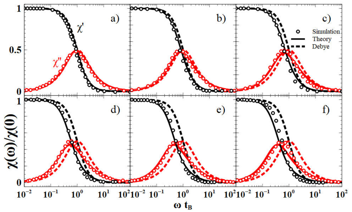
Figure 1 Semi-logarithmic plot of normalized susceptibility χ(ω)/χ(0) versus reduced frequency ωtB at six increasing values of dipole coupling: (a) λ=0.5, (b) λ=1, (c) λ=1.5, (d) λ=2, (e) λ=2.5, and (f) λ=3 and moderately concentrated ferrofluid of reduced density ρ*=0.2. The continuous lines are from theory Eq. (16) (with k = 0) which is compared with the Brownian dynamic simulations (symbol °) adapted from [²⁰]. Dash line is the Debye model, Eq. (14). Theory calculations use the Mean Spherical Approximation for the structure factor projections S,000(r). We note that theory, Eq. (16) deviates from simulations at the highest dipole coupling starting from λ=3 (see Fig. 1 (f)).  

In Fig. 2 is made the comparison of Eq. (16) (continuous lines) against the simulation data (symbol °) reported in [²⁰] for the same but higher concentrated monodisperse ferrofluid than in Fig. 1. In this plot authors of [²⁰] used a single value of dipole strength λ=1 and higher density of particles ρ*=0.6 with respect to Fig. 1. Yet, we find there is an agreement between their simulations and our model of Eq. (16). Additionally, we compared in Figs. 3 and 4, the frequency-dependent susceptibility of (16) with our original Brownian dynamic simulations.

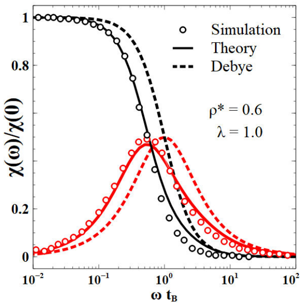
Figure 2 Frequency-dependent susceptibility χ(ω) as a function of reduced frequency ωtB. Theory of Eq. (16) (continuous line) versus simulation results (symbol °) adapted from [²⁰] depicted at the higher concentration of particles ρ*=0.6 than the system of Fig. 1, and for λ=1. The dashed line depicts the ideal paramagnetic gas. We observe that at this high concentration of particles, theory, Eq. (16), still captures all features of the simulations.  

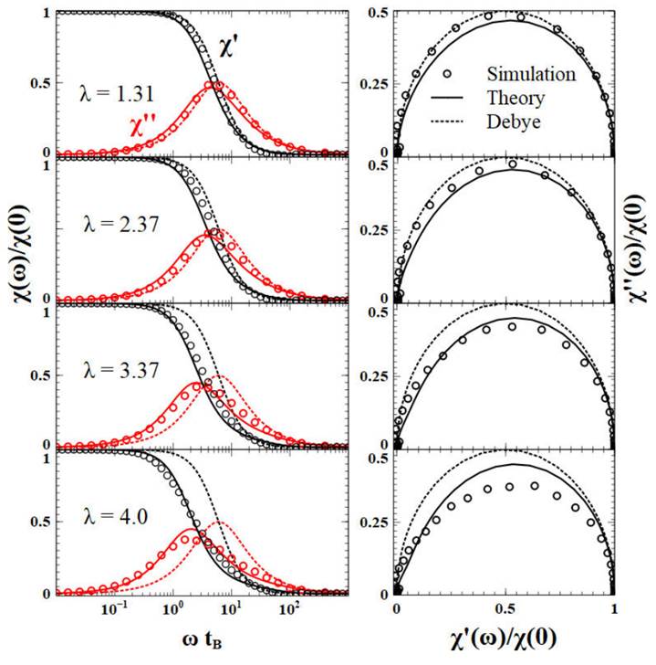
Figure 3 The semi-logarithmic plot of the Magnetic susceptibility χ(ω)/χ(0) versus dimensionless frequency ωtB. This figure provides comparisons of our original simulations (symbol °) with theory (continuous line) of Eq. (16) at k = 0 for low density of particles ρ*=0.1, and four increasing values of dipole coupling λ. The right column of panels depict the results of our simulations for the magnetic susceptibility components as Cole-Cole plots, versus theory Eq. (16). The dotted line is the ideal gas Debye theory of Eq. (14). 

Figure 4 Same properties and description as in Fig. 3 at the highest reduced density ρ*=0.9. 

In Fig. 3 depicts χ' (with black continuous line) and χ'' with gray line (red color online) for the fixed reduced density ρ*=0.1, and for increasing dipole strength λ=1.31,2.37,3.37 and 4.0, respectively. Simulation results are represented with black symbol ° for the real component of susceptibility χ', and a gray circle (red color online) for the imaginary part χ''. Whereas the dashed line symbols are the Debye theory of Eq. (14). We recall from the expression of S,mll,s(k,t) that k = 0 ignores the translational diffusion D(ω) of the magnetic particles. Therefore, there is only rotational diffusion of these interacting colloidal particles. We can observe in Fig. 3 that there is an agreement between the theory of (16) with our simulations calculations. We observe quantitative differences between them starting from the highest dipole moment λ=4.0. On the other hand, Debye theory Eq. (14) only agrees at low dipole moment λ=1.31 with Eq. (16) and simulations, see the first panel on the top of Fig. 3. This ideal Debye model deviates even more from theory (16) and our simulation results for increasing dipole moment and density.

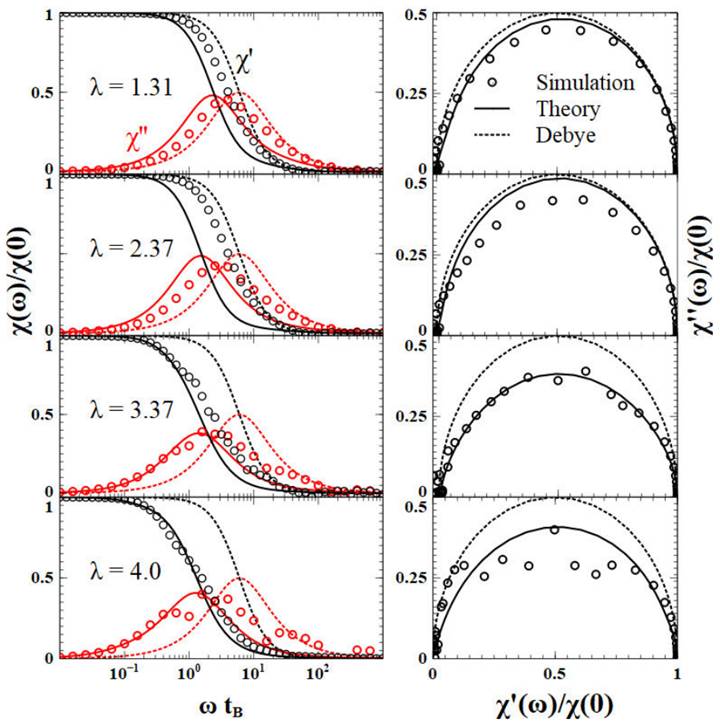
Figure 4 shows results for the case of a highly concentrated ferrofluid with ρ*=0.9.

Figures 3 and 4 include the so-called magnetic Cole-Cole plots of the imaginary component χ'' versus the real part χ' (calculated with equation (16) in the hydrodynamic limit k = 0 and plotted with black line). The symbol ° represents simulations. In these figures, we depict the Debye theory (dotted line).

In Fig. 5 are depicted comparisons of dynamic susceptibility from Eq. (16) at the hydrodynamic limit k = 0 and seven increasing values of dimensionless dipole strength λ=1.31,2.37,3.37,4,4.6,5.36,6.17 and for two reduced densities ρ*=0.1,0.5. We notice from these plots that there is a frequency shift to lower values of the imaginary contribution χ'' as the dipole moment was raised from λ=1.31 up to 4.0 where there is chain formation as observed in simulations (not depicted). Experimentally chain formation is currently observed in similar conditions [⁴¹]. Whereas the magnitude of χ' drops to lower values (the slop of the branch diminish from ωtB=0 where χ'=1 up to ωtB=103 where χ'=0) confirming qualitatively the observations of [²²]. Authors of [²²] used an ionically stabilized ferrofluid Fe₃O₄ in NaCl electrolyte solutions. They concluded that a decrease of χ' is related to particle aggregation and the frequency shift of χ'' peak is due to a larger hydrodynamic size of the cluster (chain). Remmer et al. observed similar behaviors for the susceptibility of CoFe₂O₄ nanoparticles dissolved in viscoelastic media of gelatin [²³]. Our approach can be applied to study mixtures of magnetic with non-magnetic colloids. We derived from our dynamic susceptibility model (16) its static value at ω=0. This observable was determined under the experimental condition of k→0, and in the limit of small volume fraction ϕ≪1. Under this condition on ϕ≪1 and λ≪1, the Mean Spherical Approximation for the structure factors appearing in (16) are expanded in a Taylor series expansion. The approximated expression of initial susceptibility that resulted is χϕ≈χL(1+5χL/18+11χL2/96) which differs from the known exact expression χϕ≈χL(1+χL/3+χL2/144) demonstrated by Ivanov et al. (here χL=8λϕ) [^15,16]. We compared first our approximated susceptibility with the experiments of [¹⁵] as a function of volume fraction of magnetic colloidal particles.

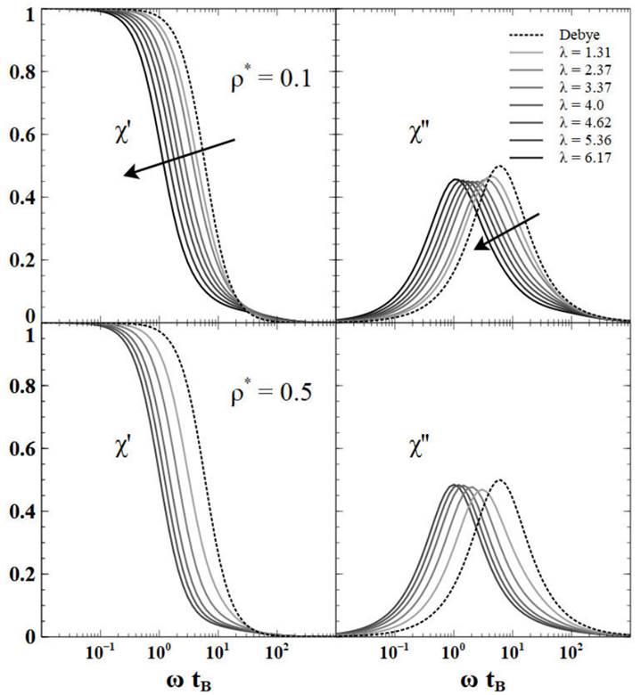
Figure 5 The semi-logarithmic plot of normalized susceptibility χ(ω)/χ(0) versus reduced frequency ωtB at two increasing values of reduced density ρ*=0.1,0.5, and seven values of increasing (denoted by the arrows’ direction) dipole coupling λ=1.31,2.37,3.37,4,4.62,5.36,6.17. We observe in these figures, a shift to lower values of the frequency in χ'' and a reduction of the slop (and amplitude) of χ' as the dipole moment per particle is increased and consequently an enhancement of the particle-particle interactions. At λ=4, there appear chain formations by the particles.  

Figure 6 compares the best fit using our expression χϕ≈χL(1+5χL/18+11χL2/96) (black line) to the experiments of the magnetic suspension studied in [¹⁵] at room temperature T = 300 K (black dots). We find that the best fit occurs with the single value λ=2.81, whereas the gray line (red color online) is the theory for the initial susceptibility χ(ω=0)=χL(1+χL/3+χL2/144) used by authors Ivanov et al. to interpret their data.

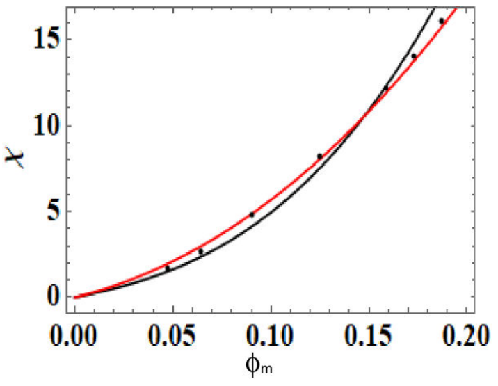
Figure 6 Initial susceptibility χ(ω=0)=χϕ as a function of the particles magnetic concentration ϕm. Black lines depicts χϕ≈χL(1+5χL/18+11χL2/96) as derived from Eq. (16) for ϕ<<1. Experiments adapted from [¹⁵] are given by symbols • for a magnetite in kerosene ferrofluid at temperature T = 300 K. Best fitting particle’s interaction strength used in the theory above was λ=2.81 and the approximation ϕ≈ϕm was used. The exact theory χ(ω=0)=χL(1+χL/3+χL2/144) adapted from [¹⁵] is depicted with grey line (red color online). Here χL=8λϕ.  

In Fig. 7 it is given the comparison of our expression of the initial susceptibility χϕ≈χL(1+5χL/18+11χL2/96) (black lines) versus temperature with those experiments of Ivanov et al. (gray lines, red color online) for their first three low volume fractions of particles (see Fig. 6 in [¹⁵]). In this case, the Langevin susceptibility χL(T) is temperature dependent, and its correction to account for this dependency is considered in [^16,15].

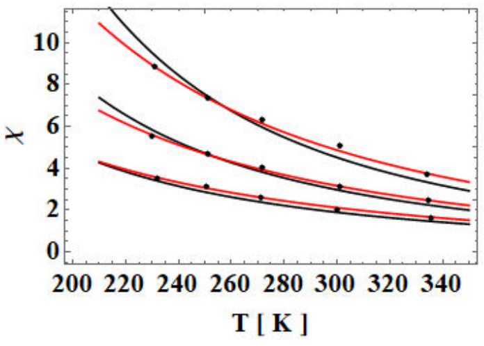
Figure 7 Initial susceptibility χ(ω=0) as a function of absolute temperature T. Black lines depict the approximated theory χϕ≈χL(T)(1+5χL(T)/18+11χL(T)2/96 derived from Eq. (16) at ϕ<<1. Experimental data with symbols • were adapted from [¹⁵]. Exact theory adapted from [¹⁵] is depicted with grey line (red color online). For the approximated theory from (16) the best fitting values to the experiments occur from top to bottom as (ϕ=0.068,λ=4.25),(0.042,2.45), and (0.12,1.4), respectively.  

Thus, our static susceptibility becomes χϕ≈χL(T)(1+5χL(T)/18+11χL(T)2/96) where χL(T)=χL(1-β1(1-ϕ)(T-T*))(1-β2T2)T*/(1-β2T*2)2 [^16,15]. The data T_* = 285 K, β1=0.87×10-3/K, β2=8×10-7/K2 were taken from the same experiments in [¹⁵]. We see that we can find qualitative agreement with the experiments of [¹⁵] by using (ϕ,λ)=(0.068,4.25),(0.092,2.45),(0.12,1.4). The gray lines (red colour online) are the results of the correct equation of Ivanov et al. χ(ω=0)=χL(T)(1+χL/3+χL2/144) which yields agreement with their data for λ=5.1,2.8,1.6 for the same ϕ as above, respectively.

5 Conclusions

In this paper, we presented the adaptation of the linear response method for the susceptibility of polar liquids to the frequency-dependent susceptibility of magnetic colloids in terms of the dynamical structure factor. Comparing the predicted initial magnetic susceptibility with existing reported experiments yields the general trends of those observations as a function of the colloid’s volume fraction and temperature. Our calculations of the magnetic susceptibility using material data of typical ferrofluids such as Fe₂O₃ yields good agreement with simulations at low dipole moments per particle and density. Finally, our approach enables us to determine magnetic susceptibility in mixtures of magnetic and non-magnetic colloids.

References

[1] E. Roeben et al., Magnetic particle nanorheology, Colloid Polym. Sci. 292 (2014) 2013. https://doi.org/10.1007/s00396-014-3289-6. [ Links ]
[2] P.C. Fannin, B.K. Scaife and S. Charles, New technique for measuring the complex susceptibility of ferrofluids, J. Phys. E Sci. Instrum. 19 (1986) 238. https://doi.org/10.1088/0022-3735/19/3/018. [ Links ]
[3] P.C. Fannin, B.K. Scaife and S. Charles, The measurement of the frequency dependent susceptibility of magnetic colloids, J. Magn. Magn. Mater. 72 (1988) 95. https://doi.org/10.1016/0304-8853(88)90276-4. [ Links ]
[4] P.C. Fannin et al., Investigation of the complex susceptibility of magnetic beads containing maghemite nanoparticles, J. Magn. Magn. Mater. 303 (2006) 147. https://doi.org/10.1016/j.jmmm.2005.07.035. [ Links ]
[5] P.C. Fannin, B.K. Scaife and S. Charles, A study of the complex susceptibility of ferrofluids and rotational Brownian motion, J. Magn. Magn. Mater. 65 (1987) 279. https://doi.org/10.1016/0304-8853(87)90051-5. [ Links ]
[6] V. Singh, V. Banerjee and M. Sharma, Journal of Physics D: Applied Physics Dynamics of magnetic nanoparticle suspensions, J. Phys. D: Appl. Phys. 42 (2009) 245006. https://doi.org/10.1088/0022-3727/42/24/245006. [ Links ]
[7] H. Mamiya, I. Nakatani and T. Furubayashi, Phase transitions of iron-nitride magnetic fluids, Phys. Rev. Lett. 84 (2000) 6106. https://doi.org/10.1103/PhysRevLett.84.6106. [ Links ]
[8] A.C. Bohórquez, C. Yang, D. Bejleri and C. Rinaldi, Rotational diffusion of magnetic nanoparticles in protein solutions, J. Colloid and Interface Sci. 506 (2017) 393. https://doi.org/10.1016/j.jcis.2017.07.009. [ Links ]
[9] B.H. Erne, K. Butter, B.W.M. Kuipers and G.J. Vroege, Rotational Diffusion in Iron Ferrofluids, Langmuir 19 (2003) 8218. https://doi.org/10.1021/la0346393. [ Links ]
[10] L. Hilger, W. Andra, R. Hergt, R. Hiergeist and W.A. Kaiser, Treatment of breast cancers by magnetic thermoablation: in vivo experiments in mice, Magnetohydrodynamics 37 ( 2001) 323. https://doi.org/10.22364/mhd.37.3.17. [ Links ]
[11] A. Jordan et al., Presentation of a New Magnetic Field Therapy System for the Treatment of Human Solid Tumors with Magnetic Fluid Hyperthermia, J. Magn. Magn. Mater. 225 (2001) 118. https://dx.doi.org/10.1016/S0304-8853(00)01239-7. [ Links ]
[12] Y.L. Raikher and V.I. Stepanov, Physical aspects of magnetic hyperthermia: Low-frequency ac field absorption in a magnetic colloid, J. Magn. Magn. Mater. 368 (2014) 421. https://doi.org/10.1016/j.jmmm.2014.01.070. [ Links ]
[13] E.L. Verde, G.T. Landi, J.A. Gomes, M.H. Sousa and A.F. Bakuzis, Magnetic hyperthermia investigation of cobalt ferrite nanoparticles: Comparison between experiment, linear response theory, and dynamic hysteresis simulations, J. Appl. Phys. 111 (2012) 123902. https://doi.org/10.1063/1.4729271. [ Links ]
[14] G.T. Landi, Role of dipolar interaction in magnetic hyperthermia, Phys. Rev. B 89 (2014) 014403. https://doi.org/10.1103/PhysRevB.89.014403. [ Links ]
[15] A.O. Ivanov et al., Temperature-dependent dynamic correlations in suspensions of magnetic nanoparticles in a broad range of concentrations: a combined experimental and theoretical study, Phys. Chem. Chem. Phys. 18 (2016) 18342. https://doi.org/10.1039/C6CP02793H. [ Links ]
[16] A.F. Pshenichnikov and A.V. Lebedev, Magnetic susceptibility of concentrated ferrocolloids, Colloid Journal 67 (2005) 189. https://doi.org/10.1007/s10595-005-0080-x. [ Links ]
[17] M.A. Martsenyuk, Y.L. Raikher and M.I. Shliomis, On the Kinetics of Magnetization of Ferromagnetic Particle Suspension, Sov. Phys. JETP 38(1974) 413. https://jetp.ras.ru/cgi-bin/dn/e-038-02-0413.pdf. [ Links ]
[18] B.U. Felderhof and R B. Jones, Mean field theory of the nonlinear response of an interacting dipolar system with rotational diffusion to an oscillating field, J. Phys.: Condens. Matter 15 (2003) 4011. https://doi.org/10.1088/0953-8984/15/23/313. [ Links ]
[19] E.S. Blums, A.O. Cebers and M.M. Maiorov, Magnetic fluids, (Walter de Gruyter, Berlin New York, 1997). [ Links ]
[20] J.O. Sindt, P.J. Camp, S.S. Kantorovich, E.A. Elfimova and A.O. Ivanov, Influence of dipolar interactions on the magnetic susceptibility spectra of ferrofluids, Phys. Rev. E 93 ( 2016) 063117. https://doi.org/10.1103/PhysRevE.93.063117. [ Links ]
[21] P. Ilg and A.E.A.S. Evangelopoulos, Magnetic susceptibility, nanorheology, and magnetoviscosity of magnetic nanoparticles in viscoelastic environments, Phys. Rev. E 97 (2018) 032610. https://doi.org/10.1103/PhysRevE.97.032610. [ Links ]
[22] S.B. Trisnanto, K. Yasuda and Y. Kitamoto, Dipolar magnetism and electrostatic repulsion of colloidal interacting nanoparticle system, Jpn. J. Appl. Phys. 57(2S2) (2018) 02CC06. https://doi.org/10.7567/JJAP.57.02CC06. [ Links ]
[23] H. Remmer, E. Roeben, A.M. Schmidt, M. Schilling and F. Ludwig, Dynamics of magnetic nanoparticles in viscoelastic media, J. Magn. Magn. Mater. 427 (2017) 331. https://doi.org/10.1016/j.jmmm.2016.10.075. [ Links ]
[24] J. Lal, D. Abernathy, L. Auvray, O. Diat and G. Grübel, Dynamics and correlations in magnetic colloidal systems studied by X-ray photon correlation spectroscopy, Eur. Phys. J. E 4 ( 2001) 263. https://doi.org/10.1007/s101890170108. [ Links ]
[25] G. Meriguet et al., Understanding the structure and the dynamics of magnetic fluids: coupling of experiment and simulation, J. Phys.: Condens. Matter 18 (2006) S2685. https://doi.org/10.1088/0953-8984/18/38/S11. [ Links ]
[26] A. Mertelj, L. Cmok and M. Copic, Anomalous diffusion in ferrofluids, Phys. Rev. E 79 (2009) 041402. https://doi.org/10.1103/PhysRevE.79.041402. [ Links ]
[27] B. Yendeti, G. Thirupati and A. Vudaygiri, Field-dependent anisotropic microrheological and microstructural properties of dilute ferrofluids, Eur. Phys. J. E 37 ( 2014) 70. https://doi.org/10.1140/epje/i2014-14070-9. [ Links ]
[28] G. Meriguet, E. Dubois, A. Bourdon, G. Demouchy and R. Perzynski, Forced Rayleigh scattering experiments in concentrated magnetic fluids: effect of interparticle interactions on the diffusion coefficient, J. Magn. Magn. Mater. 289 ( 2005) 39. https://doi.org/10.1016/j.jmmm.2004.11.012. [ Links ]
[29] F. Cousin, E. Dubois and V. Cabuil, Tuning the interactions of a magnetic colloidal suspension, Phys. Rev. E 68 (2003) 021405. https://doi.org/10.1103/PhysRevE.68.021405. [ Links ]
[30] T. Autenrieth, A. Robert, J. Wagner and G. Grübel, The dynamic behavior of magnetic colloids in suspension, J. Appl. Cryst. 40 (2007) s250. https://doi.org/10.1107/S0021889807009016. [ Links ]
[31] P. Madden and D. Kivelson, A Consistent Molecular Treatment of Dielectric Phenomena, Adv. Chem. Phys. 56 (1984) 467. https://doi.org/10.1002/9780470142806.ch5. [ Links ]
[32] D. Jiles, Introduction to Magnetism and Magnetic Materials , (Chapman and Hall/CRC, Boca Ratón Florida, 1998). [ Links ]
[33] L.G. Chambers, An Introduction to the Mathematics of Electricity and Magnetism, (Chapman and Hall, London, 1973). [ Links ]
[34] J.P. Hansen and I.R. McDonald, Theory of Simple Liquids with Applications to Soft Matter, (Academic Press, Amsterdam, 2013). [ Links ]
[35] C.G. Gray and K.E. Gubbins, Theory of Molecular Liquids, Vol. 1, (Oxford: Clarendon, Oxford, 1984). [ Links ]
[36] D. Wei and G.N. Patey, Rotational motion in molecular liquids, J. Chem. Phys. 91 (1989) 7113. https://doi.org/10.1063/1.457656. [ Links ]
[37] R. Peredo-Ortíz , M. Hernández-Contreras and R. Hernández-Gómez, Magnetic viscoelastic behavior in a colloidal ferrofluid, J. Chem. Phys. 153 (2020) 184903. https://doi.org/10.1063/5.0021186. [ Links ]
[38] R. Peredo-Ortíz and M. Hernández-Contreras, Diffusion microrheology of ferrofluids, Rev. Mex. Fis. 64 (2018). https://doi.org/10.31349/RevMexFis.64.82 82. [ Links ]
[39] S. Odenbach, Colloidal Magnetic Fluids, (Springer, Berlin, 2009). [ Links ]
[40] J. Lopez, F.J. Espinoza-Beltran, G. Zambrano, M.E. Gómez and P. Prieto, Caracterización de nanopartículas magnéticas de CoFe2o4 y CoZnFe2O4 preparadas por el metodo de coprecipitación química, Rev. Mex. Fis. 58 (2012) 293. https://rmf.smf.mx/ojs/index.php/rmf/article/view/3925. [ Links ]
[41] F. Donado, P. Miranda-Romagnoli and R. Agustín-Serrano, Phenomenological model for yield stress based on the distribution of chain lengths in a dilute magnetorheological fluid under an oscillatory magnetic field, Rev. Mex. Fis. 59 (2013). https://rmf.smf.mx/ojs/index.php/rmf/article/view/3975 131. [ Links ]
[42] U. Sandoval, J.L. Carrillo and F. Donado, Fluido magneto-reológico bajo perturbaciones magnéticas, Rev. Mex. Fis. 56 (2010) 123. https://www.scielo.org.mx/pdf/rmfe/v56n1/v56n1a14.pdf. [ Links ]
[43] S. Plimpton, Fast Parallel Algorithms for Short-Range Molecular Dynamics, J. Comp. Phys. 117 (1991) 1. https://doi.org/10.1006/jcph.1995.1039. [ Links ]
[44] M.S. Wertheim, Exact Solution of the Mean Spherical Model for Fluids of Hard Spheres with Permanent Electric Dipole Moments, J. Chem. Phys. 55 (1971) 4291. https://doi.org/10.1063/1.1676751. [ Links ]
Received: October 26, 2021; Accepted: December 10, 2021
Creative Commons License This is an open-access article distributed under the terms of the Creative Commons Attribution License