SciELO - Scientific Electronic Library Online

 
vol.68 número2Constants of motion associated with canonoid transformations for non-autonomous systemsQuasi uniformly accelered motion of quasi normal magnetic biharmonic particles in Heisenberg space with cold plasma índice de autoresíndice de assuntospesquisa de artigos
Home Pagelista alfabética de periódicos  

Serviços Personalizados

Journal

Artigo

Indicadores

Links relacionados

  • Não possue artigos similaresSimilares em SciELO

Compartilhar


Revista mexicana de física

versão impressa ISSN 0035-001X

Rev. mex. fis. vol.68 no.2 México Mar./Abr. 2022  Epub 27-Mar-2023

https://doi.org/10.31349/revmexfis.68.020707 

RESEARCH

GRAVITATION, MATHEMATICAL PHYSICS AND FIELD THEORY

Optical solitons to fractal nonlinear Schrödinger equation with non-Kerr law nonlinearity in magneto-optic waveguides

N. Razaa 

A. Yasmeena 

M. Inca 

aDepartment of Mathematics, University of the Punjab, Lahore-54590, Pakistan.


Abstract

This paper introduces the fractal model of the nonlinear Schrödinger equation with quadratic-cubic nonlinearity in magneto-optic waveguides, having plenty of applications in fiber optics. He’s variational approach and Painleve technique are used to obtain bright and kink soliton solutions of the governing system. The constraint conditions that ensure the existence of these solitons arise naturally from the model’s solution structure. To quantify the behavior of different solutions, the effect of the fractal parameter is studied. These techniques may be very useful and efficient tools for solving nonlinear fractal differential equations that emerge in mathematical physics.

Keywords: Variational principle; Painleve approach; nonlinear Schrödinger equation; solitons; quadratic-cubic nonlinearity

1. Introduction

Optical solitons are the basic component of fiber-optic telecommunication technology. Several models have been developed to investigate this mechanism, including the nonlinear Schrödinger’s equation (NLSE). There are different¨ forms of waveguides such as optical metamaterials, optical fibers and photonic crystal fibers, among others, that send a large amount of data across intercontinental distances [1,2]. This paper considers a particular type of optical waveguides with an artificially generated magnetic field, known as magneto-optic waveguides. The benefit of such waveguides is that they reduce the soliton clutter effect ensuring smooth information propagation [3-5].

In the field of nonlinear science, the NLSE is a wellknown model that can be used in a variety of physical instances, including nonlinear optics, nuclear physics, quantum mechanics, condensed matter physics, and plasma physics, etc. [6-12]. The fractal model is gaining significance in nonlinear evolution equations (NLEE) of physics and mathematics for its many attractive properties that traditional systems fail to provide. One form of fractal NLEE is coupled NLSE in nonlinear optics. This system can handle soliton solutions having applications in optical communications, logic gate devices, ultrafast soliton switches, and soliton lasers [13].

The optical soliton solutions of NLSE with various forms of nonlinearity possess a significant part in resolving realworld problems. In optics, a soliton is the wave that is unaltered during propagation due to a delicate balance between nonlinear and dispersive effects in the medium [14-16]. Solutions for various NLSE have been sought to investigate nonlinear phenomena with the solitons being either bright or dark depending on the details provided by the governing NLSE [17-20]. Researchers have been studying these solitons with quadratic-cubic nonlinearity since this form of nonlinearity was first suggested in 2011 [21]. The study of soliton dynamics in magneto-optic waveguides is crucial.

Bright solitons can be formed from a state of attraction to a state of separation from each other by magneto-optic components. This allows us to manage the so-called soliton clutter. This article explores the soliton solutions of coupled NLSE with quadratic-cubic nonlinearity by implementing He’s semi-inverse variational method and the Painlevé approach that may be conducive for engineers and physicist to physically comprehend this model.

The semi-inverse approach is an effective tool for finding different variational principles of physical problems [22,23]. He suggested the semi-inverse variational theorem as an efficient and direct algebraic approach for computing soliton solutions [24]. Many authors went on to expand this approach and contributed to the analysis of fractal models in distinct fields of science [25-28]. Another method adopted here to obtain soliton solutions of the governing model is the Painlevé approach, which is the generalization of well-known algorithms: simplest equation method, tanh-function method, and the G’/G-expansion method [29]. This is a powerful and reliable scheme to find exact solutions of NLSE by avoiding the meromorphic solutions.

The article is organized as: Section 2 is devoted to the mathematical description. Section 3 covers the study of soliton solutions of the FLE along with their graphics. Discussion of the results is presented in Sec. 4 and 5 gives the conclusion.

1.1 Governing system

The coupled model of NLSE with quadratic-cubic nonlinearity in magneto-optic waveguides is given as:

iut+l1uxx+(m1|u|+n1|u|2+p1|v|+s1|v|2)u=R1v+i(β1ux+μ1(|u|u)x+υ1(|u|)xu+η1|u|ux) (1)

ivt+l2vxx+(m2|v|+n2|v|2+p2|u|+s2|u|2)v=R2u+i(β2vx+μ2(|v|v)x+υ2(|v|)xv+η2|v|vx) (2)

where l i ,m i ,n i ,p i ,s i√ ,R i i i i and η i for i = 1,2 are constants, while i=-1. In Eqs. (1) and (2), t and x are independent and represent the temporal and spatial variables, respectively, while the dependent variables are u(x,t) and v(x,t) which show the complex valued soliton profiles. The constants l i denote chromatic dispersion, whereas m i and n i are the self-phase modulation coefficients. The cross-phase modulation is expressed by the parameters p i and s i . On the right hand side of Eqs. (1) and (2), inter-modal dispersion and the magneto-optic parameter are denoted by the coefficients β i and R i , respectively. µ i stands for self-steepening term and the coefficients of nonlinear dispersion are symbolized by υ i and η i .

2. Mathematical analysis

To continue, the initial assumptions are as follows:

u(x,t)=F1(ξ)eiχ(x,t),v(x,t)=F2(ξ)eiχ(x,t), (3)

Where

ξ=x-at,        χ(x,t)=-hx+νt+η0. (4)

Here α, h, ν and η 0 are speed, frequency, wave number, and phase constant of the wave, respectively. F i (x,t) for i = 1,2 denote the amplitude of the pulses, whereas χ(x,t) represents the phase component of the pulses.

Substituting Eqs. (3) and (4) into Eqs. (1) and (2). So, the real parts become

l1F1''-ν+l1h2+hβ1F1-R1F2

+m1-hμ1-hη1F12

+n1F13+s1F22F1+p1F2F1=0, (5)

l2F2''-ν+l2h2+hβ2F2-R2F1

+m2-hμ2-hη2F22

+n2F23+s2F12F2+p2F1F2=0, (6)

while the imaginary parts are given as:

(a+2l1h+β1)F1'+(2μ1+υ1+η1)F1F1'=0, (7)

(a+2l2h+β2)F2'+(2μ2+υ2+η2)F2F2'=0. (8)

Integrating Eqs. (7) and (8) and setting the integration constants to zero yields

(a+2l1h+β1)F1+12(2μ1+υ1+η1)F12=0, (9)

(a+2l2h+β2)F2+12(2μ2+υ2+η2)F22=0. (10)

Equating the coefficients of linearly independent functions to zero in Eqs. (9) and (10), provides the constraints:

-(2l1h+β1)=a, (11)

2μ1+υ1+η1=0, (12)

and

-(2l2h+β2)=a, (13)

2μ2+υ2+η2=0. (14)

It can be deduced from Eqs. (11) and (13) that the soliton frequency is

h=β2-β12(l1-l2), (15)

provided l 1l 2 and β 1β 2. Furthermore, we set

F1(ξ)=εF2(ξ), (16)

where ε ≠ 0,1. As a consequence, Eqs. (5) and (6) become

l1F1''-ν+l1h2+hβ1+R1εF1

+m1-hμ1+η1+εp1F12

+(n1+s1ε2)F13=0, (17)

l2εF1''-εν+l2h2+hβ2+R2F1

+ε2m2-hμ2+η2+εp2F12

+(ε3n2+s2ε)F13=0. (18)

Equations (17) and (18) are equivalent by taking the constraint conditions:

l1=εl2, (19)

n1+ε2s1=ε3n2+εs2, (20)

ν+l1h2+hβ1+R1ε=ε(ν+l2h2+hβ2)+R2, (21)

m1-h(μ1+η1)+εp1=ε2(m2-h(μ2+η2))+εp2. (22)

From the constraint Eq. (21), the wave number ν appears to be

ν=h2(εl2-l1)+h(εβ2-β1)+(R2-εR2)1-ε. (23)

Next, Eq. (17) can be rewritten as

F1''+δ1F1+δ2F12+δ3F13=0, (24)

where

δ1=-ν+l1h2+hβ1+R1εl1,

δ2=m1-hμ1+η1+εp1l1,

δ3=n1+ε2s1l1, (25)

provided l 1 ≠ 0.

In the view of [30], the fractal form of Eq. (1) and Eq. (2) can be written as:

ddξαdF1dξα+δ1F1+δ2F12+δ3F13=0, (26)

where α is the fractal dimension value and dF 1 /dξ α is the fractal derivative represented as follows:

dF1dξα=Γ(1+α)limξ-ξ0Δξ,Δξ0F1(ξ)-F1(ξ0)(ξ-ξ0)α. (27)

3. Extraction of solitons by proposed methods

3.1. Semi-inverse method

By He’s variational principle [22] we can derive the following variational formulation for Eq. (26) as:

J=Ldξ=K-Edξ

=012dF1dξα2-δ1F122-δ2F133-δ3F144dξα, (28)

where

L=12dF1dξα-δ1F122-δ2F133-δ3F144

be the Lagrangian, K = 1/2(dF 1 /dξ α ) is the kinetic energy and

E=δ1F122+δ2F133+δ3F144

is the potential energy.

Using the two scale transformation b = ξ α , Eq. (28) takes the form

J=012dF1db2-δ1F122-δ2F133-δ3F144db. (29)

Using the Ritz’s approach, consider the solitary wave solution as follows

F1=Xsech(Yb), (30)

where unknown constants X and Y are to be computed further. Substituting Eq. (30) into Eq. (29) gives

J=16X2Y-δ1X22Y-δ2πX312Y-δ3X46Y. (31)

Taking the corresponding derivatives of J with respect to X and Y gives

JX=13XY-δ1XY-δ2πX24Y-23δ3X3Y=0,    (32)

JY=16X2+12δ1X2Y2+δ2πX312Y2+16δ3X4Y2=0. (33)

From Eq. (32) and Eq. (33) we have

X=-5πδ2±25π2δ22-1152δ1δ324δ3,                   (34)

Y=±125π2δ22-πδ225π2δ22-1152δ1δ372δ3-4δ1 . (35)

Equation (30) becomes

F1=-5πδ2±25π2δ22-1152δ1δ324δ3 sech±125π2δ22-πδ225π2δ22-1152δ1δ372δ3-4δ1 b. (36)

The solitary wave solution for Eq. (26) is

u(x,t)=-5πδ2±25π2δ22-1152δ1δ324δ3 eι(hx+νt+η0)sech±125π2δ22-πδ225π2δ22-1152δ1δ372δ3-4δ1 (x-at)α, (37)

vx,t=ε-5πδ2±25π2δ22-1152δ1δ324δ3eιhx+νt+η0

×sech±125π2δ22-πδ225π2δ22-1152δ1δ372δ3-4δ1(x-at)α, (38)

provided ε ≠ 0,1.

Now, consider another possible soliton solution, this time of the form

F1=W4(Zb), (39)

where unknown constants W and Z are to be calculated later. Plugging Eq. (39) into Eq. (29) yields

J=128315W2Z-835δ1W2Z-2562079δ2W3Z-5126435δ3W4Z. (40)

Taking the corresponding derivatives of J with respect to W and Z leads to

JW=256315WZ-1635δ1WZ-256693δ2W2Z-20486435δ3W3Z=0  , (41)

JZ=128315W2+835δ1W2Z2+2562079δ2W3Z2+5126435δ3W4Z2=0  . (42)

From Eqs. (41) and (42) we have

W=-325δ2±105625δ22-486486δ1δ3504δ3  , (43)

Z=±11210325δ22-δ2105625δ22-486486δ1δ3693δ3-27δ1  , (44)

with the help of which (39) takes the form

F1=-325δ2±105625δ22-486486δ1δ3504δ3 sech±11210325δ22-δ2105625δ22-486486δ1δ3693δ3-27δ1 b. (45)

The solitary wave solution for Eq. (26) is given as:

ux,t=-325δ2±105625δ22-486486δ1δ3504δ3 eιhx+νt+η0 

×sech4±11210325δ22-δ2105625δ22-486486δ1δ3693δ3-27δ1(x-at)α, (46)

vx,t=ε-325δ2±105625δ22-486486δ1δ3504δ3eιhx+νt+η0

×sech4±11210325δ22-δ2105625δ22-486486δ1δ3693δ3-27δ1(x-at)α, (47)

provided ε ≠ 0,1.

3.2. Painlevé Approach

According to Paul Painlevé, the exact solution of Eq. (26) has the form:

F1(ξ)=e0+f(U)e-cξ,        U=g(ξ)=e1-e-cξc, (48)

and f(U) in Eq. (48) satisfies f U AU 2 = 0, which is a Riccati-equation.

The solution to this equation is given as

f(U)=1AU+U0. (49)

Differentiating Eq. (48) with respect to ξ and using Riccati equation give:

F1ξ=-ce-cξf+Ae-2cξf2,

F1ξξ=c2e-cξf-3Ace-2cξf2+2A2e-3cξf3,

F1ξξξ=-c3e-cξf+7Ac2e-2cξf2

-12A2ce-3cξf3+6A3e-4cξf4.

Substituting F 1, F 1 ξ and F 1 ξξ in Eq. (26) and comparing the coefficients of like powers of e −cξ f(U) equal to zero, we obtain the system of equations as:

2A2+δ3=0,-3Ac+δ2=0,c2+δ1=0, (50)

which implies the following four cases:

  • (i) If A=-δ3/2 and c=-δ1 then the solution is

  • F1(ξ)=e-δ1ξ-δ32U+U0.             (51)

  • (ii) If A=-δ3/2 and c=--δ1 then the solution is

  • F1(ξ)=e--δ1ξ-δ32U+U0.             (52)

  • (iii) If A=--δ3/2 and c=-δ1 then the solution is

  • F1(ξ)=e-δ1ξ--δ32U+U0.             (53)

  • (iv) If A=--δ3/2 and c=--δ1 then the solution is

  • F1(ξ)=e--δ1ξ--δ32U+U0.             (54)

TABLE I Comparison of the results following the Painlevé approach, φ6 expansion, and semi-inverse methods. 

Methods NLSE Fractal NLSE
Painlevé F1ξ=e±-δ1ξ±-δ32U+U0
ϕ6 expansion P1(ς)=(2n+1)(2n2μ1-h2)3n2μ31+(n2μ1+h2)U2(ς)3h0(fU2(ς)+g)12n
Semi-inverse qx,t=AD+coshBx-vtei-kx+ωt+θ0 u(x,t)=X[Y(x-at)α]eι(hx+νt+η0)

4.Results and discussion

The graphical interpretation of the obtained results and the effect of fractal parameter on them are discussed in this section. The semi-inverse variational method yields the bright soliton solutions given by Eqs. (37), (38), (46), and (47). The physical appearance of these solitons is shown in terms of |u|2 and |v|2 by assigning different parameteric values. In Figs.1 and 2, the 2D profiles are provided for fractal dimension values α = 0.2,0.5,0.7,0.9 while 3D plots are the standard solitary waves of Eqs. (37), (38), (46) and (47). Kink soliton solutions, i.e., Eq. (51-54) of a given model are obtained following the Painleve approach. In Figs. 3 and 4, the 3D plots of Eq. (51) and Eq. (52) are shown for distinct fractal dimension values α = 0.2,0.5,0.7,1. In Fig. 3, the oscillation spikes on the surface are due to the fractal effect. In Fig. 4, the fractal effect on the solution is shown by the irregularity in the surface. Equations (53) and (54) display the same graphical behavior with just reflection as in Figs. 3 and 4, respectively.

FIGURE 1 The 3D profile of a) Eq. (37) for |u|2 and b) Eq. (38) for |v|2 for the parameters: δ 1 = −0.12, δ 2 = 0.55, δ 3 = 1.2, π = 22/7, α = −3, α = 1, є = 1.5 2D plots of c) |u|2 and d) |v|2 against x at t = 0 for fractal dimension value α = 0.2,0.5,0.7,0.9. 

FIGURE 2 The 3D profile of a) Eq. (46) for |u|2 and b) Eq. (47) for |v|2 the parameters: δ 1 = −0.3, δ 2 = 0.55, δ 3 = 1.2, α = −3, α = 1, є = 1.5, 2D plots of c) |u|2 and d) |v|2 against x at t = 0 for fractal dimension value α = 0.2,0.5,0.7,0.9. 

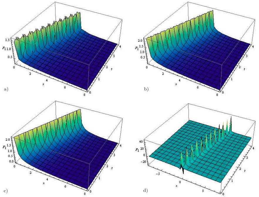
FIGURE 3 Plots of Eq. (51) for the parameters: δ 1 = −0.9, δ 3 = −2.1, α = 0.8, e 1 = 1, U 0 = 0.5 and α = 0.2,0.5,0.7,1. 

FIGURE 4 Plots of Eq. (52) for the parameters: δ 1 = −0.55, δ 3 = −2.2, α = −2, e 1 = 1, U 0 = 0.5 and α = 0.2,0.5,0.7,1. 

Remark The obtained results are compared to those existing in the literature [3, 23] and found to be novel. Kink solitons of the governing system are obtained following the Painlevé approach, while for the semi-inverse variational method we considered the fractal model of NLSE.

5.Conclusion

In this article, we have obtained the optical solitons for fractal coupled NLSE in magneto-optic waveguides that have many applications to the propagation of data in optical fibers. Bright and kink solitons are retrieved by the implementation of He’s semi-inverse and Painlevé methods. The semi-inverse approach is a fascinating integration scheme to deduce variational principles for various differential models. On the other hand, the Painlevé technique is compelling to find exact solutions of non-integrable nonlinear differential equations by averting their meromorphic solutions. The suitable choice of parameters enables us to discuss the fractal behavior of the system. The outcomes could be helpful in the telecommunication industry to increase transmission system output capability. The impact of fractal dimension value on solutions of the coupled system has been shown graphically, facilitating the understanding of understand the dynamics of the model. The applied methodologies may be conducive to solve a variety of problems arising in engineering and applied physics.

References

1 R. Fedele, H. Schamel, V.I. Karpman and P. K. Shukla, Envelope solitons of nonlinear Schrödinger equation with an anticubic nonlinearity, J. Phys. A. 36 (2003) 1169, https://doi.org/10.1088/0305-4470/36/4/322. [ Links ]

2 A.-M. Wazwaz, A study on linear and nonlinear Schrödinger equations by the variational iteration method, Chaos, Solitons Fractals 37 (2008) 1136, https://doi.org/10.1016/j.chaos.2006.10.009. [ Links ]

3 E.M.E. Zayed et al., Solitons in magneto-optic waveguides with dual-power law nonlinearity, Physics Letters A 384 (2020) 126697, https://doi.org/10.1016/j.physleta.2020.126697. [ Links ]

4 M. Savescu, A.H. Bhrawy, E.M. Hilal, A.A. Alshaery and A. Biswas, Optical solitons in magneto-optic waveguides with spatio-temporal dispersion, Frequenz 68 (2014) 9, https://doi.org/10.1515/freq-2013-0164. [ Links ]

5 M. Eslami and M. Mirzazadeh, Optical solitons with BiswasMilovic equation for power law and dual-power law nonlinearities, Nonlinear Dyn. 83 (2016) 731, https://doi.org/10.1007/s11071-015-2361-1. [ Links ]

6 G.P. Agarwal, Fiber-optic communication systems, 3th ed. (John Wiley and Sons, New York, 2002). [ Links ]

7 A.H. Khater, D.K. Callebaut, M.A. Helal and A.R. Seadawy, Variational method for the nonlinear dynamics of an elliptic magnetic stagnation line, Eur. Phys. J. D 39 (2006) 237, https://doi.org/10.1140/epjd/ e2006-00093-3. [ Links ]

8 C. Zhou and X.T. He, Stochastic diffusion of electrons in evolutive Langmuir fields, Phys. Scr. 50 (1994) 415, https://doi.org/10.1088/0031-8949/50/4/015. [ Links ]

9 I.V. Barashenkoy and V.G. Makhankov, Soliton-like “bubbles” in a system of interacting bosons, Phys. Lett. A 128 (1998) 52, https://doi.org/10.1016/0375-9601(88)91042-0. [ Links ]

10 A.K. Alomari, T.A. Jawad, D. Baleanu, K.M. Saad and Q.M. Al-Mdallal, Numerical solutions of fractional parabolic equations with generalized Mittag-Leffler kernels, Numer. Methods Partial Differ. Equ. (to be published), https://doi.org/10.1002/num.22699. [ Links ]

11 A.A. Alderremy et al., New models of fractional blood ethanol and two-cell cubic autocatalator reaction equations, Math. Methods Appl. Sci. (to be published), https://doi.org/10.1002/mma.7188. [ Links ]

12 M.M. Khader and K.M. Saad, Numerical studies of the fractional Korteweg-de Vries, Korteweg-de VriesBurgers’ and Burgers’ Equations, Proc. Natl. Acad. Sci. India A 91 (2021) 67, https://doi.org/10.1007/s40010-020-00656-2. [ Links ]

13 A. Hasegawa and Y. Kodama, Solitons in optical communications (Oxford University Press, New York, 1995). [ Links ]

14 J.F. Gómez-Aguilar et al., Optical solitons in birefringent fibers with quadratic-cubic nonlinearity using three integration architectures, AIP Adv. 11 (2021) 021521, https://doi.org/10.1063/5.0038038. [ Links ]

15 N. Raza, U. Afzal, A.R. Butt and H. Rezazadeh, Optical solitons in nematic liquid crystals with Kerr and parabolic law nonlinearities, Opt. Quantum Electron. 51 (2019) 107, https://doi.org/10.1007/s11082-019-1813-0. [ Links ]

16 N. Raza and A. Javid, Optical dark and dark-singular soliton solutions of (1+2)-dimensional chiral nonlinear Schrödinger’s equation, Waves in Random and Complex Media 29 (2019) 496, https://doi.org/10.1080/17455030.2018.1451009. [ Links ]

17 N. Raza and A. Zubair, Optical dark and singular solitons of generalized nonlinear Schrödinger’s equation with anti-cubic law of nonlinearity, Mod. Phys. Lett. B 33 (2019) 1950158, https://doi.org/10.1142/S0217984919501586. [ Links ]

18 M. Arshad, A.R. Seadawy and D. Lu, Exact brightdark solitary wave solutions of the higher-order cubicquintic nonlinear Schrödinger equation and its stability, Optik 138 (2017) 40, https://doi.org/10.1016/j.ijleo.2017.03.005. [ Links ]

19 A. Biswas et al., Resonant optical solitons with quadraticcubic nonlinearity by semi-inverse variational principle, Optik 145 (2017) 18, https://doi.org/10.1016/j.ijleo.2017.07.028. [ Links ]

20 M. Ekici et al., Solitons in magneto-optic waveguides by extended trial function scheme, Superlatt. Microstruct. 107 (2017) 197, https://doi.org/10.1016/j.spmi.2017.04.021. [ Links ]

21 J. Fujioka et al., Chaotic solitons in the quadratic-cubic nonlinear Schrödinger equation under nonlinearity management, Chaos 21 (2011) 033120, https://doi.org/10.1063/1.3629985. [ Links ]

22 J.H. He, Variational principles for some nonlinear partial differential equations with variable coefficients, Choas, Solitons Fractals 19 (2004) 847, https://doi.org/10.1016/S0960-0779(03)00265-0. [ Links ]

23 M. Asma, W.A.M. Othman, B.R. Won and A. Biswas, Optical soliton perturbation with quadratic-cubic nonlinearity by semi-inverse variational principle, Proc. Rom. Acad. A, 18 (2017) 331. [ Links ]

24 J.H. He, Some asymptotic methods for strongly nonlinear equations, Int. J. Mod. Phys. B 20 (2006) 1141, https://doi.org/10.1142/S0217979206033796. [ Links ]

25 A. Biswas et al., Optical soliton perturbation in nanofibers with improved nonlinear Schrödinger¨ equation by semi-inverse variational principle, J. Nonlinear Opt. Phys. Mater. 21 (2012) 1250054, https://doi.org/10.1142/S0218863512500543. [ Links ]

26 J. Zhang, Variational approach to solitary wave solution of the generalized Zakharov equation, Comput. Math. Appl. 54 (2007) 1043, https://doi.org/10.1016/j.camwa.2006.12.048. [ Links ]

Y. Khan, Fractal modification of complex Ginzburg-Landau model arising in the oscillating phenomena, Res. Phys. 18 (2020) 103324, https://doi.org/10.1016/j.rinp.2020.103324. [ Links ]

28 J.H. He, A fractal variational theory for one-dimensional compressible flow in a microgravity space, Fractals 28 (2020) 2050024, https://doi.org/10.1142/S0218348X20500243. [ Links ]

N.A. Kudryashov, The Painlevé approach for finding solitary wave solutions nonlinear nonintegrable differential equations, Optik 183 (2019) 642, https://doi.org/10.1016/j.ijleo.2019.02.087. [ Links ]

30 J.H. He, Fractal calculus and its geometrical explanation, Res. Phys. 10 (2018) 272, https://doi.org/10.1016/j.rinp.2018.06.011. [ Links ]

Received: March 26, 2021; Accepted: September 10, 2021

Creative Commons License This is an open-access article distributed under the terms of the Creative Commons Attribution License