


 text new page (beta)
 English (pdf)
 Article in xml format
 Article references
 Send this article by e-mail
 Cited by SciELO
  Similars in
SciELO
Similars in
SciELO 
 Permalink
1. Introduction
An ideal optical fiber has perfect circular symmetry. The polarizations are completely degenerate. Perturbations and imperfections during the fabrication process may introduce anisotropic, which are mostly of a linear or Cartesian type. Sometimes, large linear anisotropic are introduced on purpose, either by modified core geometry or by mechanical stress, to get linear polarizationmaintaining fibers, also called high-birefringence or hi-bi fibers. Bending and squeezing optical fibers does also introduce linear birefringence. Rotational effects of polarization, however, are in general less common and more difficult to produce and to understand.
In recent times, the advancement of glowing lasers and the utilization of optical fiber mechanics have attended to immense importance on flow propagation by curled fluid flows and space-curved. Exclusively torque forces of the geometric phase of isolated light anholonomy with some optical fibers have been investigated; the substance of numerous papers insensitive of their compositions are efficient or analytical. For illustration, Smith [1] examined that the torque of divergence of light generate on monochromatic optical fiber immerse bundle the supervisor is convinced by the electromagnetic fields thanks to the magnetic particle present flows in some optical fiber present transformer. It was still completed that the present is commensurate to torque, which is regular of the order of numerous scopes. Another preliminary substantiation of the geometric effect of the torque of magnetic divergence for light propagating in a magnetic optical fiber detecting a magnetic trajectory was extended [2]. Ross improved a totally geometric system to investigate the reversion in the coiled optical fiber with a fixed-torsion and endorsed its effects with several measurements in the fiber angle into a magnetic fiber. Tomita and Chiao [3] summarized the previous review of Ross for more universal fiber shapes. Also, Chiao and Wu [4] obtained a new important theoretical phase of the results of geometric phase torque. Apart from preceding researches [6-10], we request that a new electromagnetic phase with an antiferromagnetic chain.
Optical fiber investigates, phase is mostly observed by a carrier of new electromagnetic particles and their features. Some nonlinear evolution structures are frequently committed as design to establish substantially complicated scientific developments in diverse provinces of disciplines, particularly in genuine-state physics, chemical physics, plasma physics, optical physics, fluid mechanics, etcetera. Having an advanced perception of the brief substances, likewise their gradual operations in analytical operations and genuine administration in a constructive generation, it is excessively fascinating to satisfaction explicit solutions of approximately systems. Thus there endures no comprehending and unified approach to demonstrate exact solutions of all nonlinear transformation system analysts operate a diversity of diverse concepts [11-23].
It is remarkable that in numerous fields of physics, the utilizations of approximately wave interpretation and its reactions are of comprehensive importance. Traveling any wave solutions are a consequential variety of representative with some partial differential aspect and distinct nonlinear fractional differential equations (FDEs) have been established to a selection of traveling some wave improvements. Thus, flood waves are commonly immensely significant of all-instinctive phenomena; they have a superordinary elegant mathematical construction.
Fractional geometry perturbs the operations of derivatives and integrals of optional order. Over the latest several decades, it obtained enormous recognition because of its numerous modeling in distinct scientific competitions. Arbitrary-order designs are softer integer-order designs. FDEs appear in various mathematical and modeling regions comparatively physics, geophysics, polymer rheology, biophysics, capacitor theory, aerodynamics, medicine, nonlinear vibration of earthquake, supervision theory, vital fluid flow phenomena, superelasticity, and magnetical districts. For the intensive study of its utilization, we introduce comprehensive works [24-28].
The outline of the paper is organized as follows: Firstly, we consider a new theory of spherical electromagnetic radiation density with an antiferromagnetic spin of timelike spherical t-magnetic flows by the spherical Sitter frame in de Sitter space. Thus, we construct the new relationship between the new type electric and magnetic phases and spherical timelike magnetic flows de Sitter space S 1 2. Also, we give the applied geometric characterization for spherical electromagnetic radiation density. This concept also boosts to discover of some physical and geometrical characterizations belonging to the particle. Moreover, the solution of the fractionalorder systems is considered for the submitted mathematical designs. Graphical demonstrations for fractional solutions are presented to the expression of the approach. The collected results illustrate that mechanism is a relevant and decisive approach to recover numerical solutions of our new fractional equations. Components of performed equations are demonstrated by using approximately explicit values of physical assertions on received solutions. Finally, we construct that electromagnetic fluid propagation along fractional optical fiber indicates a fascinating family of fractional evolution equations with diverse physical and applied geometric modeling in de Sitter space S 1 2.
2. Timelike spherical t − magnetic particle in
S 1 2
In this section, the orthonormal frame design is explained by the orthonormal Lorentzian new spherical Sitter frame and the particle γ : I → S 1 2 refreshing this spherical Sitter frame equation is defined as Lorentzian spherical particle.
where ∇ is a Levi-Civita form and ε = det(Ψ, t ,∇, t) is curvature of particle [19]. Then products of spherical vector fields are presented by
Assume that γ : I → S 1 2 be a timelike spherical t-magnetic particle and G be the magnetic field in S 1 2 Timelike spherical t-magnetic particle is defined by
*Lorentz force ϕ of a t-magnetic particle with the magnetic field G is presented by
where β = h(ϕ(γ), n).
Putting force equation
where
Let γ(s,t) is the evolution of t-magnetic particle in de Sitter space. The flow of t-magnetic particle is given by
where χ 1 ,χ 2 are potentials.
Time derivatives of the spherical frame are produced by
∗ Condition of Lorentz forces ϕ(γ), ϕ(t), ϕ(n) and magnetic field G t for a rotational equilibrium of the timelike t-magnetic particle
where β = h(ϕ(γ), n).
∗In this way, the equation for Lorentz forces ϕ(γ), ϕ(T), ϕ(N) reads
where
3. New geometric results with physical applications
The geometric density theory, or the theory of density systems, has had and has an enormous impact in applied physical mathematics and an extensive diversity of nonlinear phenomena in mathematical physics. This framework combines questions in nonlinear flux optics, field designs and sigma models, fluid dynamics, relativity, electromagnetic wave theory. In this section, we obtain spherical electric and magnetic radiation density conditions by using Heisenberg antiferromagnetic model.
♣ Spherical electric and magnetic radiation density are given by
♣ By using density, a new type of spherical electric and magnetic phase is given by
New type spherical electric and magnetic phase of ϕ(γ)
Theorem 1. The spherical electric and magnetic phase of ϕ(γ) are given by
Proof. Definition of magnetic antiferromagnetic spin is given by
Then, it is easy to see that
Straightforward computations lead to
On the other hand, the magnetic-total phase along Lorentz force ϕ(γ) is indicated by
With some calculations, we have
Magnetic anholonomy density of ϕ(γ) is given by
Also, we present
Spherical electric and magnetic radiation density are given by
By magnetic anholonomy density with an antiferromagnetic model is obtained
After antiferromagnetic condition, we obtain
By this way, we conclude
Similarly, we can easily obtain that
As a reaction, we get the following impressive results.
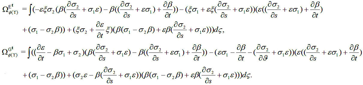
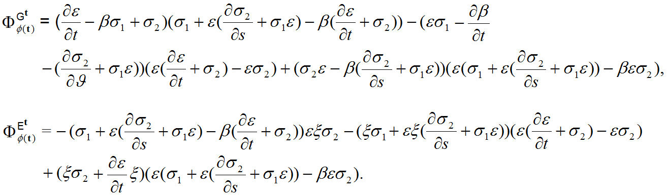
Theorem 2. Electromagnetic radiation density of ϕ(γ) is
Theorem 3. The antiferromagnetic spherical electric and magnetic phase of ϕ(γ) with antiferromagnetic spin are given by
Proof. Spherical electric and magnetic radiation density with an antiferromagnetic model are given by
If we use above theorem, we may give the following corollary:
Corollary 1. Electromagnetic radiation density with an antiferromagnetic model is
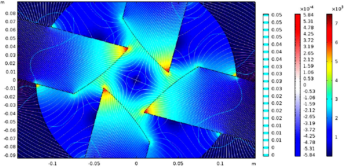
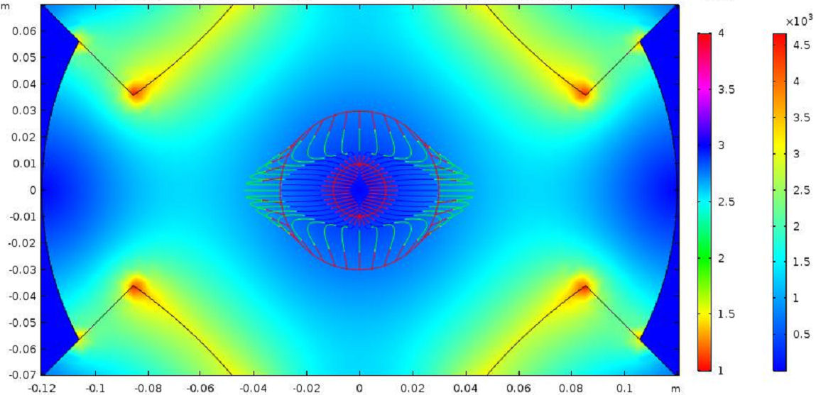
Spherical magnetic anholonomy density and time like t-magnetic particle flows in kernel of magnetic quadrupole for timelike spherical evolution with Lorentz force ϕ(γ). Spherical antiferromagnetic density is provided by the antiferromagnetic density algorithm in Fig. 1.
Magnetic antiferromagnetic spin for ϕ(t)
Theorem 4. Spherical electric and magnetic phase of ϕ(t) are given by
Proof. Magnetic antiferromagnetic spin is given by
By definition, we get
Furthermore, we have that
The previous system becomes
Magnetic total spherical phase for force ϕ(t) is obtained by
We can immediately check that
Hence, we compute
From the magnetic total phase, we obtain
It follows that
Similar to the above, we calculate
This implies that
As a reaction, we get the following impressive results.
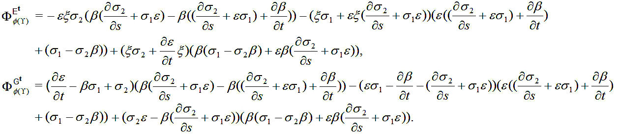
Theorem 5. The electromagnetic radiation density of ϕ(t) is
Theorem 6. Antiferromagnetic spherical electric and magnetic phase of ϕ(t) are given by
Proof. Spherical electric and magnetic radiation density with an antiferromagnetic model are given by
Under the antiferromagnetic condition, then we obtain that
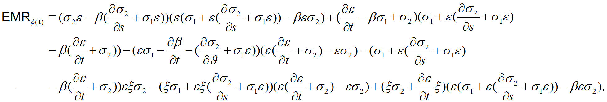
Corollary 2. Electromagnetic radiation density with an antiferromagnetic model is
Spherical magnetic anholonomy density and timelike t-magnetic particle flow in the kernel of magnetic quadrupole for timelike spherical evolution with Lorentz force ϕ(t). Spherical antiferromagnetic density is provided by the antiferromagnetic density algorithm in Fig. 2.
Magnetic antiferromagnetic spin for ϕ(n)
Theorem 7. Spherical electric and magnetic phase of ϕ(n) are given by
Proof. From spherical Sitter frame, we obtain
We instantly calculate
Combining the above relations, we get
Magnetic total spherical phase for spherical Lorentz force ϕ(n) is presented by
Consequently, we have
By further calculation, we have that
These equations are equivalent to
We immediately compute
By using a spherical Sitter frame, we give
We immediately compute the density, namely
Since, we instantly arrive at
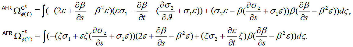
As a reaction, we get the following impressive results.
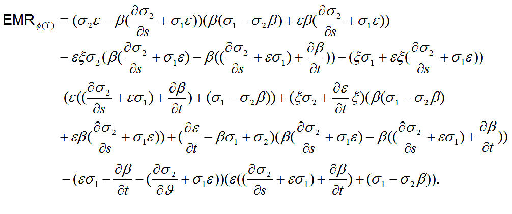
Theorem 8. The electromagnetic radiation density of ϕ(n) is
Theorem 9. Antiferromagnetic spherical electric and magnetic phase of ϕ(n) are given by
Proof. By antiferromagnetic model, we get
Spherical electric and magnetic radiation density with an antiferromagnetic model are given by
Corollary 1. Electromagnetic radiation density with an antiferromagnetic model is
Spherical magnetic anholonomy density and timelike t-magnetic particle flow in the kernel of magnetic quadrupole for timelike spherical spherical evolution with Lorentz force ϕ(n). Spherical antiferromagnetic density is provided by antiferromagnetic density algorithm in Fig. 3.
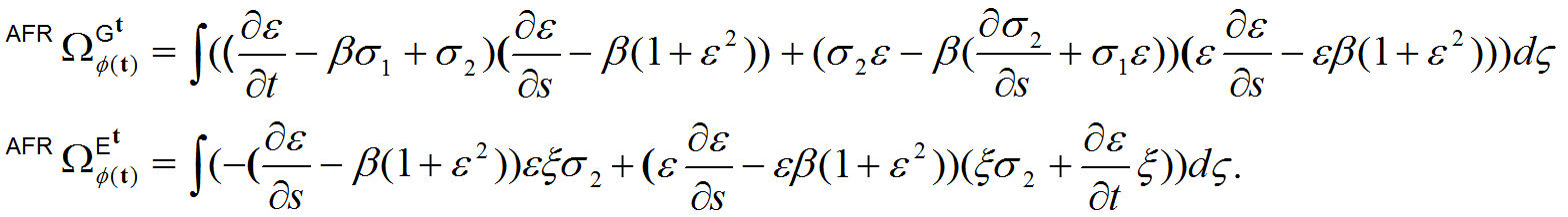
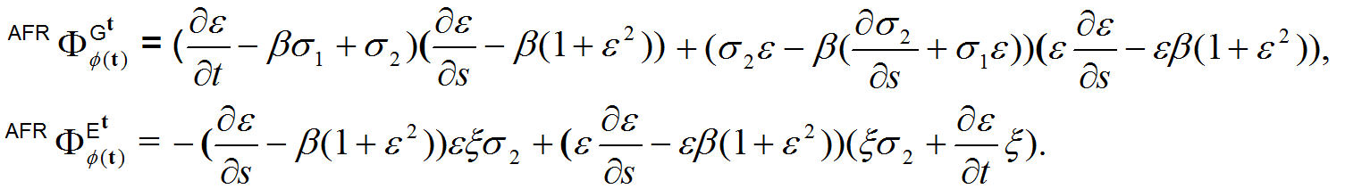
4. Optical Soliton for Extended direct algebraic method with Fractional Equation in S 1 2
In this section, we design perturbed fractional solutions of the nonlinear evolution equation governing the propagation of solitons by magnetic fields of the polarized light ray traveling in spherical fractional optical fiber. The traveling assumption concept is operated to gauge analytical soliton solutions. Then numerical duplications are also contributed to complement the rational outcomes. Also, we deal with the following evolution equations of Lorentz force ϕ(n).
where
The conformable derivative of order η ∈ (0,1] is defined as the subsequent interpretation [23]
Some of the components of conformable derivatives are in such a way [29,30].
• Assume that the traveling wave variable is
By using u(ϕ) and v(ϕ), we have
• Recognize the solution of Eqs. (4.4),
where α n ≠0, β n ≠0 and G(ϕ) can be defined as:
where ϑ,χ,f are arbitrary fixeds.
Some solutions of Eq. (4.6) are given by:
1) If χ 2 − 4ϑf < 0 and f≠0, then
2) If χ 2 − 4ϑf > 0 and f≠0, then
3) If ϑf > 0 and f = 0, then
4) If ϑf < 0 and χ = 0, then
5) If ϑ = f and χ = 0, then
6) If ϑ = −f and χ = 0, then
7) If χ 2 = 4ϑf, then
8) If χ = k, ϑ = mk, (m≠0) and f = 0, then
9) If χ = f = 0, then
10) If χ = ϑ = 0, then
11) If ϑ = 0, and χ ≠ 0 , then
12) If
Remark. The generalized hyperbolic and triangular functions are defined [29];
By placing the above equations, we have
The solutions of the above equation be a finite series as follows:
where G(ϕ) satisfies Eq. (4.6)
Putting
where G(ϕ) satisfied Eq. (4.6).
Also, solving the above system, we get
New solutions of Eq. (4.1) are presented by:
1) If χ 2 − 4ϑf < 0 and f≠0, then
2) If χ 2 − 4ϑf > 0 and f≠0, then singular soliton and dark solutions are presented by
3) If ϑf > 0 and χ = 0, then the singular new periodic solutions are presented by
5) If ϑ = f and χ = 0, then singular new periodic solutions are presented by
6) If ϑ = −f and χ = 0, then dark and singular soliton new solutions are presented by
7) If χ 2 = 4ϑf, then rational new solution is presented by
8) If χ = k, ϑ = mk (m≠0) and f = 0, then the rational solution is presented by
9) If χ = f = 0, then rational new solution is presented by
10) If χ = ϑ = 0, then rational new solution is presented by
11) If ϑ = 0, and χ≠0, then dark like new solitons are presented by
12) If χ = k, and ϑ = 0 and f = mk (m≠0), then rational new solution is presented by
5. Graphical representation of the solutions
The magnetic flow graphics of the performed solutions are demonstrated in the illustrates by applying Mathematica. In Figs. 4-5, we produce some numerical simulations of ε(s,t) and σ 2(s,t) in 3D plots when 0 ≤ s ≤ 5 and 0 ≤ t ≤ 5.
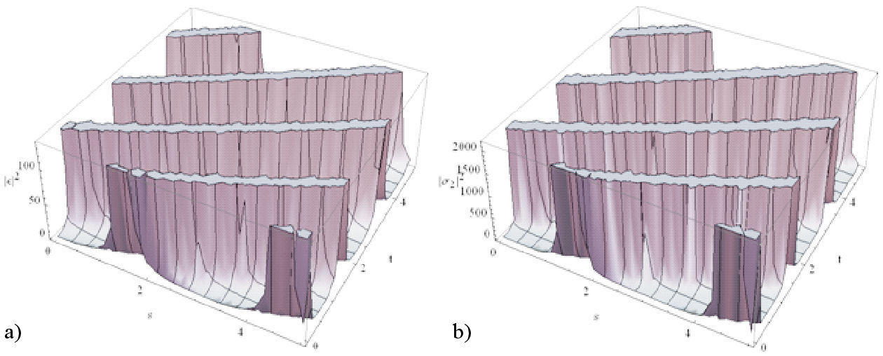
FIGURE 4 The magnetic flow graphics for the analitical solutions of the fractional (4.1) equations (h = f = 2, χ = 1) a) ε 1(s,t), b) σ 21(s,t).
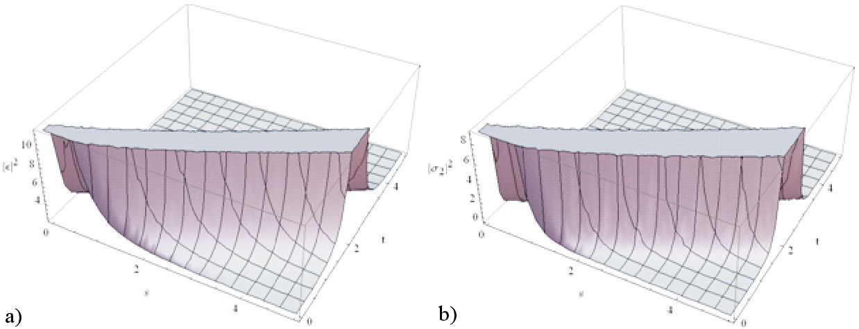
FIGURE 5 The magnetic flow graphics for the analitical solutions of the fractional (4.1) equations (h = −2, f = 1, χ = 0) a) ε 5(s,t), b) σ 25(s,t).
We displayed the some of solutions recovered for the presented fractional (4.1) equations by a conformable derivative operator. Besides, we showed 3D graphics for some of the solutions in Figs. 4-5. The above figures were drawn for A = 1.7, η = 0.8, ∆ = Ω = 1.
6. Conclusion
Geometrical models that describe a relativistic magnetic particle may be constructed using the geometrical scalars associated with the embedding of the particle worldline in Heisenberg spacetime as building blocks for the action. In this investigation, we consider a new theory of optical magnetic spherical antiferromagnetic spin of timelike spherical magnetic flows of the t-magnetic particle by the spherical Sitter frame in de Sitter space. Also, the extended direct algebraic method is used to find new soliton solutions of the fractional (4.1) equations in de Sitter space. Many partial differential equations are proceeding in mathematical physics and engineering modeling applications [31-46]. We express that the suggested approach is applicable to investigate the plenty of illustrations based on engineering and science.

