SciELO - Scientific Electronic Library Online

 
vol.67 número5Soliton solution of generalized Zakharov-Kuznetsov and Zakharov-Kuznetsov-Benjamin-Bona-Mahony equations with conformable temporal evolutionTime-dependent SI model for epidemiology and applications to Covid-19 índice de autoresíndice de materiabúsqueda de artículos
Home Pagelista alfabética de revistas  

Servicios Personalizados

Revista

Articulo

Indicadores

Links relacionados

  • No hay artículos similaresSimilares en SciELO

Compartir


Revista mexicana de física

versión impresa ISSN 0035-001X

Rev. mex. fis. vol.67 no.5 México sep./oct. 2021  Epub 28-Mar-2022

https://doi.org/10.31349/revmexfis.67.050707 

Research

Gravitation, Mathematical Physics and Field Theory

Two reliable techniques for solving conformable space-time fractional PHI-4 model arising in nuclear physics via β-derivative

B. Elma a  

E. Misirli b  

aEge University, Department of Mathematics, İIzmir/Turkey. e-mail: berfin-elma@hotmail.com

bEge University, Department of Mathematics, İzmir/ Turkey. e-mail: emine.misirli@ege.edu.tr; emine.misirli@gmail.com


Abstract

Nowadays, nonlinear fractional partial differential equations have been extensively used to model physical phenomena. It is very important to achieve exact solutions of fractional differential equations for understanding complex phenomena in mathematical physics, and therefore, studies on fractional differential equations have increased. In this study, new exact traveling wave solutions of the space-time fractional Phi-4 equation have been achieved by using two powerful different techniques, and solutions have additionally been checked. The space-time fractional Phi-4 equation has been expressed through Atangana’s conformable derivative. Obtaining new solutions to this equation shows that methods are effective to ascertain other nonlinear complex problems in particle and nuclear physics.

Keywords: The functional variable method; the first integral method; fractional Phi-4 equation; traveling wave solutions; beta-derivative

1. Introduction

Studies on fractional differential equations have recently increased to model some complex phenomena more accurately. There are many different definitions of fractional derivatives in literature. Some of them are the Caputo derivative [1], the Caputo-Fabrizio derivative [2], the Riemann-Liouville derivative [1], Jumarie’s modified Riemann-Liouville derivative [3], and Atangana-Baleanu derivative [4]. Fractional partial differential equations (FPDEs) have been used in various areas such as physics, control theory, biology, mathematical physics, applied mathematics, optics, chemistry [5-10].

In this article, two reliable methods have been applied to reach the exact solutions of the fractional Phi-4 equation with Atangana’s beta-derivative. One of the methods is the functional variable method [11-12] and the other one is first integral method [13-14]. In some applications in literature, various techniques have been applied to FPDEs [15-26].

The paper is organized as follows: Some basic definitions and properties of Atangana’s beta-derivative are introduced in Sec. 2. In Sec. 3, the functional variable method and the first integral method are examined in detail. In Sec. 4, methods are applied to the fractional Phi-4 equation to obtain some new exact solutions. The final section includes a conclusion containing all outputs in this article.

2. Definition of Atangana’s beta-derivative

Definition 1: Let h : [0,∞) → R be a function. Then its fractional conformable derivative of h order α is,

D0Atαgt=limε0hx+εx1-α-hxε, (1)

Khalil et al. defined the above theorem for the fractional derivatives [27].

However, there are similar features between conformable fractional derivatives and ordinary derivatives. For instance, the product derivative and the quotient derivative of two functions. Thus, mathematicians, physicists, and engineers have made many studies on conformable derivatives [28]. Definition 2: Atangana’s beta-derivative is as following

D0Atαgt=limε0g(t+ε[t+1Γα]1-α)-gtε. (2)

Atangana’s derivative allows us to remove some weak properties of the conformable derivative. For example; A differentiable function’s derivative is equal to zero at the zero points [29]. Thanks to beta derivative, real-world problems which arise in applied mathematics and physics are modeled more accurately. Thus, the physical behavior of the graphics can be interpreted more precisely.

Atangana’s derivative can be preferred because it provides the maximum properties of the fundamental derivatives. Some important features for Atangana’s beta derivatives [30]:

Let us take h 6= 0 and g are two function differentiable with β-order and β ∈ (0,1]. Then

D0Axα{agx+bhx}=aD0Axα{gx}+bD0Axα{hx}   for   a,bR. (3)

For any dR. Then,

D0Axα{d}=0 (4)

Dxα{d}{gxhx}=hx0ADxα{gx}+gx0ADxα{hx}. (5)

D0Axα{gxhx}=hx0ADxα{gx}+gx0ADxα{hx}h2x (6)

Using Eq. (2), ε = (x + (1/Γ(α))) 1−α f, if ε → 0 then f → 0. The Eq. (7) has been obtained.

D0Axα{gx}=(x+1Γα)1-αdgxdx, (7)

and

μ=γα(x+1Γα)α, (8)

where γ is a constant. Finally, we can write the following equation

D0Axα{gμ}=γdgμdμ. (9)

3. Description of methods

3.1. Functional variable method (FVM)

A brief description of the suggested method:

Step 1. FPDE can be written in the form:

F(u,D0Atα,D0Axαu,ux,ut,)=0. (10)

Step 2. Using wave transformation

ux,t=Uξ, (11)

ξ=kα(x+1Γα)α-γα(t+1Γα)α. (12)

Taking into account Eq. (12), we reduce the FPDE to a nonlinear ordinary differential equation:

PUξ,U'ξ,U''ξ,=0 (13)

where U (ξ) = dU(ξ)/dξ.

P is a polynomial of U and its derivatives while u ξ = du/dξ, u ξξ = d 2 u/dξ 2 and so on.

Step 3. We introduce a functional variable for making a new transformation to unknown function U

uξ=Fu (14)

and some successive derivatives of u(ξ) to following:

uξξ=12F2'uξξξ=12F2''F2,uξξξξ=12([F2]'''F2+12[F2]''[F2]'). (15)

Step 4. After substituting (14) and (15) into (13) the ODE can be reduced as

Ru,F,F',F'',=0. (16)

After integration, Eq. (16) provides the expression of F, and this gives the appropriate solutions to the original problem, together with Eq. (14).

3.2. First integral method (FIM)

A summary of the FIM is presented,

Step 1. FPDE can be written in the form:

F(u,D0Atαu,D0Axαu,ux,ut,)=0. (17)

Step 2. Using wave transformation

ux,t=Uξ, (18)

ξ=kα(x+1Γα)α-γα(t+1Γα)α. (19)

Taking into account Eq. (19), we reduce the FPDE to a nonlinear ordinary differential equation:

PUξ,U'ξ,U''ξ,=0, (20)

where U () = dU(ξ)/dξ.

Step 3. Afterwards, defining some new independent variables

Uξ=Xξ,Uξξ=Yξ, (21)

then we get a new system of the following form:

Xξ=Yξ,Yξ=GXξ,Yξ. (22)

Step 4. By using the division theorem, we can reach a first integral to Eq. (22). The exact solutions of Eq. (17) are obtained by solving this equation.

Division Theorem: Suppose that R(x,y) and Q(x,y) are polynomials in C[x,y]; and R(x,y) is irreducible in C[x,y]. If Q(x,y) vanishes at all zero points of R(x,y), then there exists a polynomial H(x,y) in C[x,y] such that

Qx,y=Rx,y.Hx,y.

4. Solution of the space-time fractional Phi-4 equation

The conformable space-time fractional Phi-4 equation [31]:

D0At2αu,D0Ax2βu+m2u+n3u=0,0<α,β1, (23)

0ADtαu indicates the Atangana’s conformable fractional derivative of u with respect to t of order α and m, n are real constants.

Using the following transformation:

ux,t=Uξ,ξ=lβx+1Γββ-λαt+1Γαα, (24)

where ξ is the transformation variable and l,λ be the constants. Eq. (23) changes into the form an ordinary differential equation:

λ2U''ξ-l2U''ξ+m2Uξ+nU3ξ=0. (25)

4.1. Solution by functional variable method

Equation (25) can be written as follows:

Uξξ=m2l2-λ2U+nl2-λ2U3. (26)

Then we use the transformation u ξξ = (1/2)(F 2) in in Eq. (15), we get Eq. (27) from Eq. (26)

F2'=2m2l2-λ2u+2nl2-λ2u3. (27)

Integrating (27) with respect to u and we obtain

Fu=n2l2-λ2uu2+2m2n. (28)

From (14) and (28), we deduce that

duuu22m2n=n2l2-λ2ξ+ξ0, (29)

where ξ 0 is a integration constant. After integrating (29), we have the following exact solutions:

Case 1. If 2m 2 /n > 0 ⇒ m = 0, then

u1x,t=±1n2l2-λ2(lβx+1Γβββ-λαt+1Γαα+ξ0). (30)

Case 2. If 2m 2 /n > 0 ⇒ m = 0, then

u2x,t=2m2ncschml2-λ2lβx+1Γββ-λαt+1Γαα+ξ0, (31)

u3x,t=-2m2ncschml2-λ2lβx+1Γββ-λαt+1Γαα+ξ0, (32)

u4x,t=2m2nsechml2-λ2lβx+1Γββ-λαt+1Γαα+ξ0 (33)

u5x,t=-2m2nsechml2-λ2lβx+1Γββ-λαt+1Γαα+ξ0. (34)

Case 3. If 2m 2 < 0, then

u6x,t=-2m2ncscmλ2-l2lβx+1Γββ-λαt+1Γαα+ξ0, (35)

u7x,t=--2m2ncscmλ2-l2lβx+1Γββ-λαt+1Γαα+ξ0, (36)

u8x,t=-2m2nsecmλ2-l2lβx+1Γββ-λαt+1Γαα+ξ0, (37)

u9x,t=--2m2nsecmλ2-l2lβx+1Γββ-λαt+1Γαα+ξ0. (38)

4.2. Solution by first integral method

Using Eq. (21) and Eq. (22), we can write two dimensional autonomous system

dXdξ=YξdYdξ=m2l2-λ2Xξ-nl2-λ2X3ξ. (39)

According to the first integral method, we suppose that X and Y are non-trivial solutions of the Eq. (39). Also, Q(X,Y)=i=0mai(X)Yi is an irreducible polynomial in C[X,Y ], such that

QXξ,Yξ=i=0maiXξYiξ=0, (40)

where a m (X) 6= 0 and i = 0,1,...,m. By division theorem ∃ a polyn. g(X) + h(X)Y , such that

dQdξ=dQdXdXdξ+dQdYdYdξ=gX+hXYi=0maiXYi. (41)

Assume that m = 1 then coefficients of Y i(i = 0,1) in Eq. (40), we have:

a1'X=a1XhX, (42)

a0'=a0XhX+a1XgX, (43)

 a1X(m2l2-λ2X-nl2-λ2X3)=a0XgX. (44)

Since a i (X) are polynomials, then we deduce that a 1(X) is constant and h(X) = 0. Let us take a 1(X) = 1 and for the equilibrium of a 0(X) and g(X) degrees, deg(g(X)) = 1. Suppose that g(X) = A 0 + A 1 X and we find

a0X=A0X+12A1X2+C, (45)

where C is the integration constant. We obtain a nonlinear system of the algebraic equations from a 0(X), g(X), and Eq. (44).

A1=2nl2-λ2l2-λ2,C=m22nl2-λ2  A0=0, (46)

And

A1=-2nl2-λ2l2-λ2,C=-m22nl2-λ2  A0=0. (47)

Under the conditions given by Eqs. (46) and (47) in Eq. (40), we have,

Yξ=±(m22nl2-λ2+2nl2-λ22l2-λ2X2ξ). (48)

Using Eq. (48) and Eq. (11), we can convert to Eq. (48) following Ricatti equation

U'ξ=±(m22nl2-λ2+2nl2-λ22l2-λ2U2ξ). (49)

Some special solutions are achieved:

Type 1. If 1/(l 2λ 2) > 0, then

u10x,t=m2ntanm22l2-λ2lβx+1Γββ-λαt+1Γαα+ξ0, (50)

u11x,t=-m2ntanm22l2-λ2lβx+1Γββ-λαt+1Γαα+ξ0, (51)

u12x,t=m2ncotm22l2-λ2lβx+1Γββ-λαt+1Γαα+ξ0, (52)

u13x,t=-m2ncotm22l2-λ2lβx+1Γββ-λαt+1Γαα+ξ0. (53)

Type 2. If 1/(l 2λ 2) < 0, then

u14(x,t)=-m2ntanh(m22(λ2-l2)[lβ{x+1Γ(β)}β-λαt+1Γαα+ξ0]), (54)

u15(x,t)=--m2ntanh(m22(λ2-l2)[lβ{x+1Γ(β)}β-λαt+1Γαα+ξ0]), (55)

u16(x,t)=-m2ncoth(m22(λ2-l2)[lβ{x+1Γ(β)}β-λαt+1Γαα+ξ0]), (56)

u17(x,t)=--m2ncoth(m22(λ2-l2)[lβ{x+1Γ(β)}β-λαt+1Γαα+ξ0]). (57)

5. Graphical representations

5.1. Graphs of solutions with FVM

FIGURE 1 Graph of of u 1 for n = 1.7, λ = 0.2 and l = −1.5.  

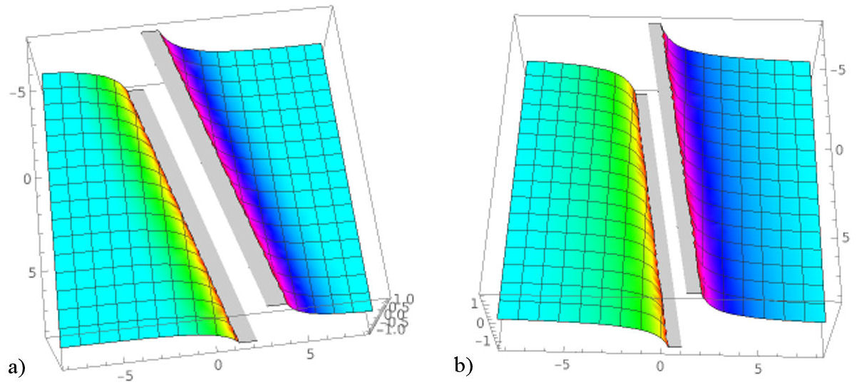
FIGURE 2 a) Graph of u 2 for m = −0.6, n = 1.06, λ = −0.2 and l = −0.7. b) Graph of u 2 for m = −0.2, n = 1.7, λ = −0.1 and l = −0.7. 

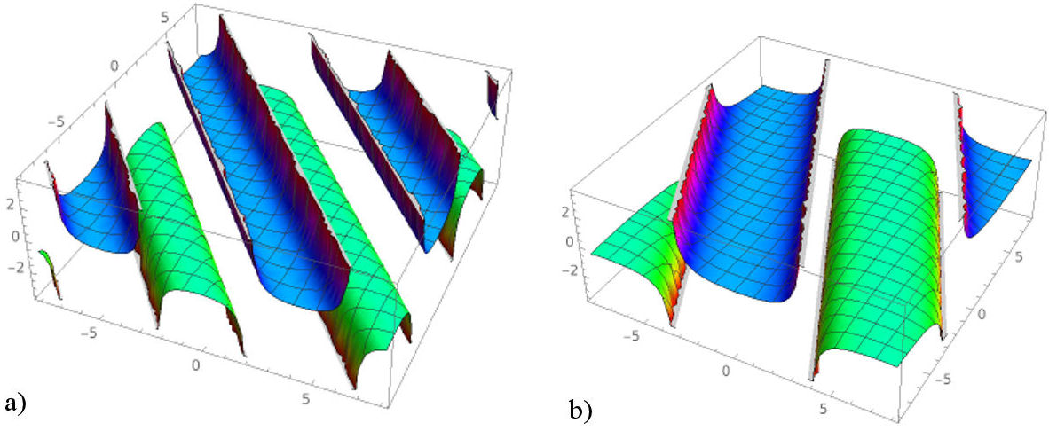
FIGURE 3 a) Graph of u 4 for m = −0.8, n = 0.3, λ = −0.4 and l = 0.9. b) Graph of u 4 for m = −0.8, n = 0.6, λ = −1 and l = 1.3. 

FIGURE 4 a) Graph of u 6 for m = −0.4, n = −1.3, λ = 0.9 and l = −1.1 b) Graph of u 6 for m = −0.4, n = −1.3, λ = 0.5 and l = −1.1. 

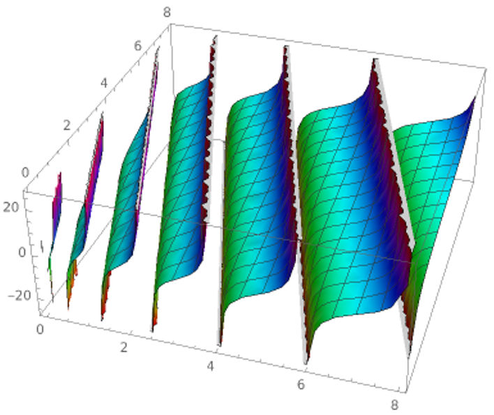
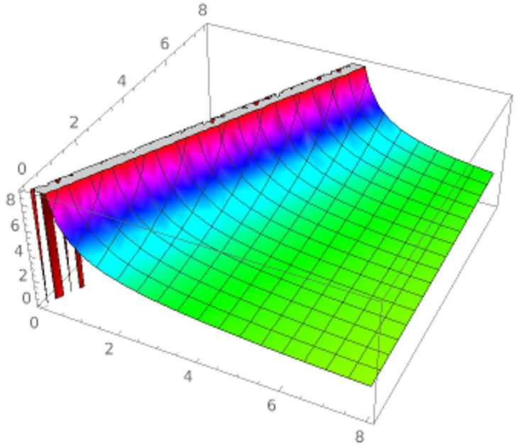
5.2. Graphs of solutions with FIM

In this section, 3D graphs of the solutions have been included. Some specific parameters have been chosen to reach different types of wave graphs. Figures 2, 3, and 4 can give an opinion about the physical behavior of solutions based on the change of amplitude and width of the waves. While periodic solutions, hyperbolic solutions and rational solutions have been achieved by using FVM (Figs. 1-4), hyperbolic solutions, and trigonometric solutions have been obtained by using FIM (Figs. 5-8). The first method gives compacton waves and bell-shaped soliton waves whereas the second one gives compacton waves and kink soliton waves. Thanks to these powerful methods, different types of solutions can be helpful to understand the physical behavior of other nonlinear FPDEs in mathematical and nuclear physics.

FIGURE 5 Graph of u 10 for m = −3.2, n = 0.51, λ = −2.98 and l = 3.03. 

FIGURE 6 Graph of u 12 for m = 1.17, n = −0.57, λ = 1.96 and l = 4.36. 

FIGURE 7 Graph of u 15 for m = 1.64, n = −2.72, λ = 1.7 and l = −2.45. 

FIGURE 8 Graph ofu 17 for m = −0.83, n = 1.4, λ = −0.96 and l = 4.14. 

6. Conclusions

In this paper, two powerful and reliable analytical techniques have been applied to Atangana’s conformable space-time fractional Phi-4 equation. Tha main advantage of FVM is its wide applicability. The main idea of FIM is reducing fractional partial differential equation to ordinary differential equation and then generating the first integral with the help of division theorem. The idea shows that the FIM is concisely direct. Thanks to FVM and FIM, we have obtained more solution functions than the other famous analytical methods. All solution functions have been checked by using the Mathematica program. Additionally, physical behaviors of solution functions have been examined for some appropriate values of the parameters. Results show that the proposed methods are very effective, straightforward, and strong to solve nonlinear FPDEs defined by Atangana’s derivative.

References

1. I. Podlubny, Fractional Differential Equations: an Introduction to Fractional Derivatives, Fractional Differential Equations, to Methods of Their Solution and Some of Their Applications. Elsevier, (1998). [ Links ]

2. M. Caputo, M. Fabrizio, A new definition of fractional derivative without singular kernel. Progr. Fract. Differ. Appl, 1 (2015) 1-13. DOI: https://doi.org/10.1016/j.aml.2019.02.033 [ Links ]

3. C. Li, Q. Guo, M. Zhao, On the solutions of (2 + 1)-dimensional time-fractional equation. Appl. Math. Lett., 94 (2019) 238-243. [ Links ]

4. A. Atangana and D. Baleanu, New fractional derivatives with nonlocal and non-singular kernel: theory and application to heat transfer model. Therm. Sci., 20 (2016) 763. DOI: 10.2298/TSCI160111018A [ Links ]

5. K.S. Miller, B. Ross, An Introduction to the Fractional Calculus and Fractional Differential Equations. John Wiley, New York, (1993). [ Links ]

6. M. Senol, O. Tasbozan, A. Kurt, Numerical Solutions of Fractional Burgers’ Type Equations with Conformable Derivative. Chinese Journal of Physics, 58 (2019) 75-84. DOI: 10.1016/j.cjph.2019.01.001 [ Links ]

7. S. Sarwar, S. Iqbal, Stability analysis, dynamical behavior and analytical solutions of nonlinear fractional differential system arising in chemical reaction. Chinese Journal of Physics , 56 (2018) 374-384. https://doi.org/10.1016/j.cjph.2017.11.009 [ Links ]

8. R.L. Magin, Fractional Calculus in Bioengineering, Begell-House Publisher, 125 West Redding. Conn, (2006). [ Links ]

9. V.F. Morales-Delgado, M.A. Taneco-Hernández, J.F. Gómez-Aguilar, On the solutions of fractional order of evolution equations. The European Physical Journal Plus, 132 (2017) 1-14. https://doi.org/10.1140/epjp/i2017-11341-0 [ Links ]

10. A. Atangana, J.F. Gómez-Aguilar , Decolonisation of fractional calculus rules: Breaking commutativity and associativity to capture more natural phenomena. The European Physical Journal Plus , 133 (2018) 1-22. DOI : https://doi.org/10.1140/epjp/i2018-12021-3 [ Links ]

11. E. M. E. Zayed, Y. A. Amer, A. H. Arnous, The functional variable method and its applications for finding the exact solutions of nonlinear PDEs in mathematical physics. Scientific Research and Essays, 8 (2013) 2068-2074. https://doi.org/10.5897/SRE2013.5725 [ Links ]

12. Y. Yıldırım et al., Pure-cubic optical soliton perturbation with full nonlinearity. Optik, 222 (2020) 165394. https://doi.org/10.1016/j.ijleo.2020.165394 [ Links ]

13. M. Eslami, H. Rezazadeh, The first integral method for Wu-Zhang system with conformable time - fractional derivative. Calcolo, 53 (2016) 475-485. https://doi.org/10.1007/s10092-015-0158-8 [ Links ]

14. M. Eslami , F. S. Khodadad, F. Nazari, H. Rezazadeh , The first integral method applied to the Bogoyavlenskii equations by means of conformable fractional derivative. Optical and Quantum Electronics, 49 (391) (2017). https://doi.org/10.1007/s11082-017-1224-z [ Links ]

15. A.A. Gaber, A.F. Aljohani, A. Ebaid and J. Tenreiro Machado, The generalized Kudryashov method for nonlinear space-time fractional partial differential equations of Burgers type. Nonlinear Dyn., 95 (2019) 361. https://doi.org/10.1007/s11071-018-4568-4 [ Links ]

16. Y. Pandir, Y. Gurefe and E. Misirli, The extended trial equation method for some time-fractional differential equations. Discrete Dyn. Nat. Soc., 2013 (2013) 491359. https://doi. org/10.1155/2013/491359 14 [ Links ]

17. Y. Pandir , Y. Gurefe andE. Misirli , New exact solutions of the time-fractional Nonlinear dispersive KdV equation. Int. J. Model. Opt., 3 (2013) 349. DOI: 10.7763/IJMO.2013. V3.296 [ Links ]

18. A. Kurt , O. Tasbozan , and Y. Cenesiz, Homotopy analysis method for conformable burgers-korteweg-de vries equation. Bull. Math. Sci. Appl, 17 (2016) 23. DOI: 10.18052/www.scipress.com/BMSA.17.17 [ Links ]

19. A. Zafar, Rational exponential solutions of conformable space-time fractional equal-width equations. Nonlinear Engineering, (2018). https://doi.org/10.1515/nleng-2018-0076 [ Links ]

20. D. Kumar, K. Hosseini, and F. Samadani, The sine-gordon expansion method to look for the traveling wave solutions of the tzitzéica type equations in nonlinear optics. Optik-International Journal for Light and Electron Optics, 149 (2017) 446. https://doi.org/10.1016/j.ijleo.2017.09.066 [ Links ]

21. S. Zhang, Q.A. Zhong, Fractional sub-equation method and its applications to nonlinear PDE’s. Physics Letters A 375 (2011) 1069-1073. DOI:10.1016/j.physleta.2011.01.02 [ Links ]

22. O. Guner, A. Bekir, H. Bilgil, A note on exp-function method combined with complex transform method applied to fractional differential equations. Advances in Nonlinear Analysis, 4 (2015) 201-208. DOI:10.1515/anona-2015-0019 [ Links ]

23. K. Kamruzzaman, M. A. Akbar, Exact solutions of the (2+1)-dimensional cubic Klein-Gordon equation and the (3+1)-dimensional Zakharov200 Kuznetsov equation using the modified simple equation method. J. Assoc. Arab Univ. Basic Appl., 15 (2014) 74-81. https://doi.org/10.1016/j.jaubas.2013.05.001 [ Links ]

24. K. Hosseini , A. Bekir , R. Ansari, Exact solutions of nonlinear conformable time-fractional Boussinesq equations using the (−ϕ(ε)) - expansion method. Opt Quant Electron. 49 (2017) 13. https://doi.org/10.1007/s11082-017-0968-9 [ Links ]

25. Y. Jiang, J. Ma, High-order finite element methods for time-fractional partial differential equations. J. Comput. Appl. Math., 235 (2011) 3285-3290. https://doi.org/10.1016/j.cam.2011.01.011 [ Links ]

26. J.-S. Duan, T. Chaolu, R. Rach, Solutions of the initial value problem for nonlinear fractional ordinary differential equations by the Rach-Adomian-Meyers modified decomposition method. Appl. Math. Comput. 218 (2012) 8370-8392. DOI: 10.1016/j.amc.2012.01.063 [ Links ]

27. R. Khalil, M. Al Horani, A. Yousef, M. Sababheh, A new definition of fractional derivative. Journal of Computational and Applied Mathematics, 264 (2014) 65-70. DOI: 10.1016/j.cam.2014.01.002 [ Links ]

28. R. OZARSLAN, Conformable Derivative Approach to Gross Domestic Product Model with Real Data of World Bank. Bilecik Şeyh Edebali Üniversitesi Fen Bilimleri Dergisi, 7 (2020) 1-9. https://doi.org/10.35193/bseufbd.640361 [ Links ]

29. H. Yépez-Martínez, J.F. Gómez-Aguilar, Fractional sub-equation method for Hirota-Satsuma-coupled KdV equation and coupled mKdV equation using the Atangana’s conformable derivative. Waves in Random and Complex Media, 29 (2019) 678-693. https://doi.org/10.1080/17455030.2018.1464233 [ Links ]

30. Y. Gurefe , The generalized Kudryashov method for the nonlinear fractional partial differential equations with the beta-derivative. Rev. Mex. Fis, 66 (2020) 771-781. https://doi.org/10.31349/RevMexFis.66.771 [ Links ]

31. U. Khan, R. Ellahi, R. Khan, S.T. Mohyud-Din, Extracting new solitary wave solutions of Benny - Luke equation and Phi- 4 equation of fractional order by using (G’/G) - expansion method. Optical and Quantum Electronics , 49 (2017) 362. DOI: 10.1016/j.amc.2012.01.063 [ Links ]

Received: January 11, 2021; Accepted: February 18, 2021

Creative Commons License This is an open-access article distributed under the terms of the Creative Commons Attribution License