


 text new page (beta)
 English (pdf)
 Article in xml format
 Article references
 Send this article by e-mail
 Cited by SciELO
  Similars in
SciELO
Similars in
SciELO 
 Permalink
1.Introduction
The ongoing COVID-19 epidemic represents a global challenge for health-care systems. The SARS-COV-2 coronavirus causing the COVID-19 is highly transmissible 1,2. Nevertheless, the epidemic propagation in a region/country is influenced by several factors, including governmental measures 3. The Cuban government has implemented several strategies of social isolation to control this epidemic. As a result, a small number of cases is reported in the province of Santiago de Cuba. Mathematical models are useful for understanding the COVID-19 transmission and the influence of government interventions 4-7. Currie et al. 4 suggest that system dynamics (differential-equation-based modeling) is suitable to model government decisions that cause social distancing and isolation.
The most common system dynamics in epidemic modeling are SIR (susceptible - infectious - removed) and SEIR (susceptible-exposed-infectious-removed) type. The classic SIR and SEIR models assume that individuals change classes (e.g., from susceptible to infected) at constant rates. This assumption is not realistic in most situations 8. Additionally, it does not explain why the effective reproduction number of COVID-19 changes over time 9. Some authors introduce time-dependent parameters to formulate realistic models of the current pandemic 5 10-12.
A challenge for COVID-19 modelers is to describe the difference between total cases and diagnosed cases. One approach is to exclude this difference and fit the model to reported data 16-8. Another option is to consider undetected cases as a compartment of the differential equations system 6,7,12,19,20. Finally, some authors avoid the complication of adding a new compartment, and they model the error with different ad hoc methods 5,10,21,22.
Mathematical models have been used to forecast the dynamics of COVID-19 in delimited geographical areas. These models usually fit big-number data after several days of epidemic evolution 7,10,23-26. The official data reported from Santiago de Cuba show a maximum value of 36 active cases reached 31 days after the first confirmed case. This peak is followed by a decreasing trend. These small and noisy data make difficult the model fitting. A common strategy to describe COVID-19 dynamics is to update one or more model parameters based on key days of government actions 7,10,12.
Ordinary differential equation (ODE) based models are widely used to capture the kinetic of biological systems and to predict the behaviour of time-dependent variables. The minimization of a cost function (as a strategy for fitting a given dynamic model) does not take into account the uncertainty of parameters. Additionally, this approach can lead to unrealistic fittings 27.
Bayesian inference offers a platform that deals naturally with both problems, but it requires the calculation of likelihood functions 13-15,28. In many practical problems, likelihood functions become analytically intractable; nevertheless, data can be simulated from a parameter vector by applying some algorithm that depends on the model. Thus, several techniques have been developed to infer parameters without using likelihood functions. These techniques are usually called approximate Bayesian computation (ABC) or free likelihood inference 28,29.
ABC can be used to estimate parameters when the available data of an infectious disease is coarse 30. Besides, ABC accomplishes parameters estimation for models that include dedicated laws to describe the error between total cases and reported cases.
The aim of this paper is to adapt two models reported in the literature to capture the dynamics of the noisy and small-number data of COVID-19 in Santiago de Cuba. For this, we modify an extended SEIR model (10) by introducing a dynamic-mode gamma distribution to describe the error between total and reported cases. Additionally, we adapt the classic SIR model reported in 31 by introducing Poisson noise in the observation of removed cases. For both models, we update a parameter on critical days of government actions and estimate the parameter values with ABC. We are not aware that these modifications have been reported in the literature.
2.Methods
2.1.Data
Because no personal data of patients were used, the ethical approval and individual consent were not applicable.
We used official data of cumulative, infected, and removed cases of COVID-19 in Santiago de Cuba province. These data were reported from March 20th to May 4th, 2020. Daily data was provided by the Provincial Direction of Public Health of Santiago de Cuba and visualized in an information board from a web platform (http://www.covid19scu.uo.edu.cu). Forty-nine patients with SARS-COV-2 were confirmed using real-time polymerase chain reaction (PCR) tests. PCR tests were made in the Laboratory of Molecular Biology, Provincial Center of Hygiene, Epidemiology and Microbiology of Santiago de Cuba.
2.2.Epidemiological evidence
The first day of the COVID-19 in Santiago de Cuba province counted when the first case was diagnosed (March 17th, 2020). The first case (day one), the second case (day four), and the third case (day seven) were contacts of different travelers from various countries with COVID-19 transmission reported. The number of diagnosed cases increased from day seven and they were contacts of three first confirmed cases. The epidemiological investigation revealed that the primary infectious focus was small in Santiago de Cuba province due to the small number of travelers that arrived in this province. All confirmed cases with COVID-19 were attended and treated in the Dr. José Joaquín Castillo Duany hospital of Santiago de Cuba. The confirmed patients remained at least 14 days admitted to the hospital. When two PCR tests were negative, patients were sent home under medical supervision. Additionally, all contacts of these confirmed patients were quickly isolated during 14 days to detect symptomatic and non-symptomatic cases. After 14 days of isolation, unconfirmed cases of COVID-19 were sent home and daily evaluated by physicians.
The government of Santiago de Cuba took different actions that restrained COVID-19 transmission, such as the urban and interprovincial travel restrictions; workers were encouraged to work from their homes; safe transportation was provided for essential people in the different prioritized activities; school activity was temporarily suspended at all educational levels; social movement was restrained; and the modified quarantine was established on the case clusters of importance for disease transmission.
2.3.Methodology
In order to understand and predict COVID-19 in Santiago de Cuba, we have chosen two deterministic models: one more explanatory and the other more parsimonious. The first model allowed to elaborate hypotheses about some possible causes of the few reported cases. The second model was used to make faster and accurate predictions of the epidemic evolution. For both models, we updated a parameter on key days of government action. Also, we included error models to explain the variability of the observed data. Details of the chosen models are shown in the following section.
2.4.Models
Lin et al. 10 reported an SEIR model with three additional classes: the total population size (N), the public perception of risk (D), and the cumulative cases number (C). Also, they modeled the zoonotic transmission during the first month and then only person-to-person transmission, taking into account the emigration rate inside the country.
Unlike 10, we did not consider the zoonotic transmission because infection in Cuba was not originated by animals. Also, we neglected the emigration rate for two reasons: first, the few days elapsed before the transport restriction by air, land, and sea; second, the social isolation actions taken, such as remote work, stopping school activities, among others. As a result of these two assumptions, we obtained the following model, named model-I:
with
where
To describe the error in reported data, we assumed that the difference CT - CR between total cases (CT) and reported cases (CR) is a gamma probability distribution. The assumption of a discrete random variable as a continuous one provided some advantages in the assessment of parameter estimation. For instance, it was possible to perform a nonparametric continuous hypothesis test over residues. The shape parameter of the gamma distribution was estimated, and the scale parameter was changed dynamically. This approach allowed us to place the mode closer to zero in the most optimistic scenarios. We used an incremental error in the reported rate during the early days of the epidemic. A dedicated law was formulated for the number of unreported cases per each reported one (U(t)), given by
where p and δ are tuning parameters and dT is the time from which COVID-19 transmission showed higher regularity in the case count. We empirically set the values in p = 0.01 day-1, δ = 0.04 and dT = 8 days. We assumed that U(t) increased during the days when almost no new cases arose, and after that, it remained roughly constant. This assumption is consistent with a previous study that reported growth in undocumented cases during the early days of the epidemic. The expression for the dynamic mode of error (M(t)) is
The difference between CT and M(t) was considered a time-dependent approximation of undetected cases.
Model-II consisted of a standard SIR model 31, adapted with the introduction of Poisson noise in the removed cases. For the parameter calibration of model-II, reported cumulative and removed cases were considered. We described β(t) in the model-II as a stepwise function that included changes in key dates. The error was assumed as a standard normal distribution for model-II.
2.5.Parameter estimation
Parameter estimation was performed with the ABC approach 28,33,34. We preferred the sequential Monte Carlo (ABC SMC) method described in the Algorithm 4.8 of 34 because of its well-documented results. Nevertheless, the ABC SMC method can perform slowly computing adaptive tolerances.
This sampler (Algorithm 1 in Appendix A) outsmarts its predecessors in automatic computing of tolerances based on the effective sample size of the previous population. We used N = 104, h0 = 108, T = 5 and a Gaussian acceptance kernel function Kh. We refer readers to for a deeper understanding of ABC samplers and their adjustable parameters.
The reweight step of the chosen ABC SMC sampler led to an optimization problem in the calculation of hm. Thus, it may introduce delays in the computation process, especially if the posterior distribution is distant from the prior distribution. Therefore, we introduced the hybrid version of ABC techniques, named ABC H algorithm (Algorithm 2 in Appendix B) as a hybrid of rejection sampler (ABC RS) and Markov chain Monte Carlo (ABC MCMC) approaches. Although we have not demonstrated the ergodicity of the ABC H algorithm, we empirically ascertained that it found a maximum-a-posteriori (MAP) located within the parameter region determined by the ABC SMC algorithm, consuming less computational time. Hence, we preferred to use the MAPs obtained by the ABC H sampler for quick prediction and the ABC SMC process for more in-depth posterior Bayesian analysis. Specifically, we used the ABC SMC results to compute the credible intervals of posterior distributions. Details of the algorithms ABC SMC and ABC H are shown in A and B, respectively.
As far as we know, the ABC H sampler is a new idea, and its main disadvantage may
be the inaccuracy of the sampling from the posterior distribution. This issue
was not critical because we aimed to give a quick prediction based on the MAP.
Nevertheless, we hypothesize that for a reasonably high value assigned to the
fourth sampling choice (w3, corresponding to a conventional ABC
MCMC), it is possible to obtain posterior distributions similar to ABC SMC
results. Further research is required to verify this hypothesis. We used the
scheme
Because actual data can be directly compared to simulated data for ODE models, it was not necessary to use summary statistics as criteria of divergence. We used the sum of squared errors as the distance criterion, which is closely related to the likelihood 33,35,36, and suitable for infectious-disease modeling 30. We used a methodology for the prior-distribution choice that consisted of several trials mimicking different favorable and unfavorable scenarios, followed by feedback from epidemiologists.
Values of d = 0.2 and σ = 1/3 day-1 in model-I were reported in 10. The remaining parameter values and the initial conditions E(0) and D(0)were estimated with ABC starting from locally uniform prior distributions.
In our approach, two key dates of travel restrictions divided the evolution of the epidemic into three periods. Three governmental action strengths were estimated for these periods: before travel restrictions (α1), after interprovincial travel restriction (α2), and after the urban public transport restriction in Santiago de Cuba (α3). The three values β1, β2, and β3 were considered in model-II taking into account the same criteria for key dates mentioned above.
We calculated the coefficient of determination R2 for the regression analysis of MAP fit to assess the quality of parameter-estimation results for models I and II. We performed the frequentist and nonparametric Mann-Whitney U test , taking as null hypothesis that the actual residues obtained arose from the assumed gamma distribution. Furthermore, an approximation of maximum likelihood (ML) ratio between models (ML of model-I to ML of model-II) was computed with ABC output.2
All simulations were made in a 256-core high-performance-computing (HPC) processor with 256 GB RAM using Python 3.6 39. The HPC machine was acquired by the Flemish Development Cooperation through VLIR-UOS (Flemish Interuniversity Council-University Cooperation for Development of Belgium) in the context of the Institutional University Cooperation program with Universidad de Oriente, Santiago de Cuba.
3.Results
Model-I simulation (Fig. 1) was performed with MAPs calculated with ABC SMC. All parameters and results of model-I fitting are summarized in Table I. The Mann-Whitney U test performed on the residues of model-I fit did not reject the null hypothesis based on a 5% significance level.
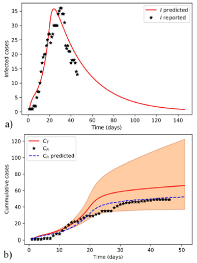
Figure 1 Estimated evolution of COVID-19 epidemic in Santiago de Cuba with model-I. The selected parameter values for simulation correspond to the MAP of the approximate posterior distribution. The model-predicted and reported infected individuals a), and the cumulative b), both predicted in simulation (C T and C R predicted) and observed (C R ) cases are plotted. The shaded area is limited by the extremes of 95% credible intervals of posterior distributions obtained with the ABC SMC sampler.
Table I Summary table of model-I parameters and results.
| Parameter | Notation | Prior or fixed value | MAP (ABC SMC) | MAP (ABC H) |
| Transmission rate |
β0 α1 |
U (0.1, 1.5) |
0.4811 days-1 CI(0.3680, 0.5468) 0.5245 |
0.4340 days-1 0.6179 |
| Fitting parameter | α2 | U (0.1, 1) |
CI(0.3717, 0.7534) 0.2855 |
0.1801 |
| α3 |
CI(0.1775, 0.3692) 0.9665 |
0.9417 | ||
| Intensity of responds | k | U (600, 4000) |
CI(0.8527, 1.0000) 3430 |
3405 |
| CI(3335, 3598) | ||||
| Mean latent period | σ-1 |
3 days U (1, 40) |
- 21 days | - 25 days |
| Mean infectious period | γ-1 | |||
| Proportion of severe cases | d | 0.2 | - | - |
| Mean duration of public reaction | λ -1 | U(30,30) | 20 days | 50 days |
| public reaction Initial susceptible | S(0) | 9.41 · 105 | CI(1, 39) - | - |
| population | ||||
| Initial exposed | E(0) | U (1, 10) | 6 | 6 |
| population | CI(4, 7) | |||
| Initial infectious | I(0) | 1 | - | - |
| population | ||||
| Initial removed | R(0) | 0 | - | - |
| population | ||||
| Initial risk perception | D(0) | U (1, 103) | 163 | 148 |
| CI(142, 188) | ||||
| Initial cumulative cases | C(0) | 1 | - | - |
Figure 2 was obtained using the MAPs of posterior distributions of model-II parameters that were computed with ABC SMC. These MAPs and other values from model-II are summarized in Table II.
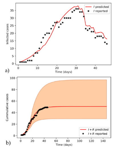
Figure 2 Estimated evolution of COVID-19 epidemic in Santiago de Cuba with model-II. Predicted infected individuals follow the dynamics of the reported ones a). A long-term scenario of both reported and predicted cumulative cases, and the area limited by the extremes of the 95% credible intervals of posterior distributions obtained with the ABC SMC sampler b) are plotted.
Table II Summary table of model-II parameters.
| Parameter | Notation | Prior or fixed value | MAP (ABC SMC) | MAP (ABC H) |
| β1 | 0.5674 days-1 | 0.5149 days-1 | ||
| Transmission rate | β2 | U (0.1, 0.9) |
CI(0.3067, 0.7534) 0.5855 days-1 |
0.6056 days-1 |
| β3 |
CI(0.4794, 0.7088) 0.3555 days-1 |
0.3548 days-1 | ||
| Mean infectious period | γ-1 | U (1, 10) |
CI(0.2443, 0.4525) 2 days |
2 days |
| CI(1, 3) | ||||
| Interval expectation | λ | U (1, 20) | 18 days | 18 days |
| of removed Initial susceptible | S(0) | 9.41x10⁵ | CI(12, 23) - | - |
| population | ||||
| Initial infectious | I(0) | 1 | - | - |
| population | ||||
| Initial removed | R(0) | 0 | - | - |
| population |
In all trials made, the ABC H sampler consumed less time and reached similar parameter regions to the ones obtained by ABC SMC (Figs. 3-6) for the same prior distributions.
Model-I predicted a total of 73 infected at the end of the COVID-19 epidemic in Santiago de Cuba, with 21% of undocumented cases. The final value of M(t) was 57, being the model-I prediction of confirmed cases. Model-II forecasted 51 confirmed cases at the end of the epidemic. Additionally, the ML ratio calculated was 0.941; and the values of determination coefficients were R2 = 0.9450 for model-I and R2 = 0.9781 for model-II.
4.Discussion
COVID-19 dynamics in Santiago de Cuba is difficult to capture empirically without the introduction of stepwise functions for parameter 𝛼 in model-I and parameter β in model-II. Results show that model-I (Fig. 1) and model-II (Fig. 2), fitted with ABC algorithms, can predict an early small-number peak of infected cases and the approximate ending of the COVID-19 in Santiago de Cuba. The non-rejection of the null hypothesis on the residuals allows us to continue considering the validity of the error law for model-I.
All MAPs calculated with ABC H are within credible intervals obtained with ABC SMC,
except parameter λ of model-I. Even for this parameter, the histogram generated by
ABC H partially overlapped the one generated by ABC SMC. We deduce that both
algorithms find the same parameter region for the chosen prior. A visual comparison
of Fig. 3 with Fig. 4, and Fig. 5 with Fig. 6, reveals that ABC H does not sample from
the same distribution as ABC SMC. Although this does not affect the use of ABC H in
this work, a modification of the ABC H sampler is required to make it a fully
functional ABC algorithm. The scheme
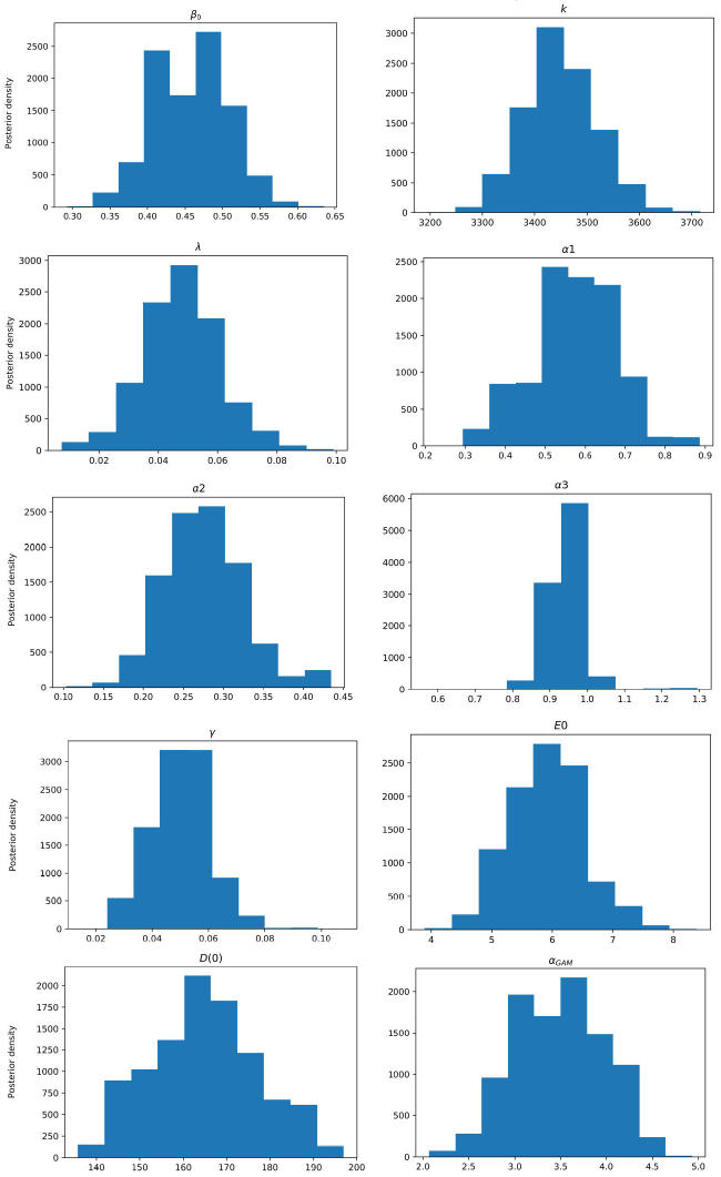
Figure 3 Posterior density estimation of model-I parameters using ABC SMC sampler and COVID-19 data from Santiago de Cuba. The estimated parameters are β0, k, λ, α1, α2, α3, γ, E(0), and the scale parameter of the gamma distribution (α GAM ).
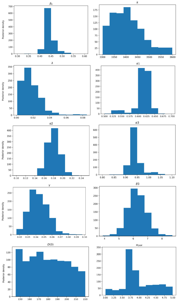
Figure 4 Posterior density estimation of model-I parameters using ABC H sampler and COVID-19 data from Santiago de Cuba. The estimated parameters are β0, k, λ, α1, α2, α3, γ, E(0), and the scale parameter of the gamma distribution α GAM .
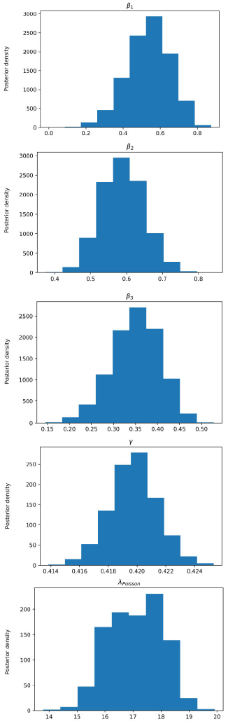
Figure 5 Posterior density estimation of model-II parameters using ABC SMC sampler and COVID-19 data from Santiago de Cuba. The estimated parameters are β1, β2, β3, γ, and the interval expectation of the Poisson distribution (λPoisson).
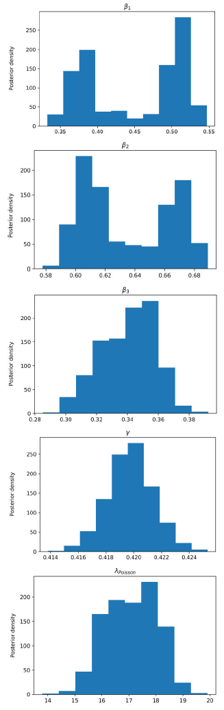
Figure 6 Posterior density estimation of model-II parameters using ABC H sampler and COVID-19 data from Santiago de Cuba. The estimated parameters are β1, β2, β3, γ, and the interval expectation of the Poisson distribution (λPoisson).
The computed percentage of undocumented cases is in contrast with the 86% of unreported infected cases estimated for China 43. This result suggests that the limited progression of the COVID-19 epidemic in Santiago de Cuba may be due to opportune epidemiological investigations, effective control measures in each source of infection, and a low number of initially exposed individuals (E(0) = 6). Additionally, case clusters prevail over transmission clusters for COVID-19 in Santiago de Cuba province. The policymakers used these estimates to complement an investigation into the initial infectious load of SARS-COV-2 in Santiago de Cuba.
The MAPs of a posterior distributions were estimated at α = 0.5245, α2 = 0.2855, and α3 = 0.9665 (Table I). Value of 𝛼 is expected to grow as government measures increase but, surprisingly, the value after the closure of transportation between provinces is lower than before (α2 < α1). We consider two possible explanations for this result:
First, the interpretation of α as government action is somewhat forced. In a previous study 42, α was interpreted as seasonality of transmission associated with the school calendar for a similar formulation of β(t). Consequently, the interpretation of α remains open.
Second, the increase in PCR tests coincides with the period corresponding to α2. Neither the deterministic model nor the error law explicitly takes into account the variability of PCR tests. This variability influences the number of detected cases, and therefore the estimation of all transmission-rate parameters.
Thus, in our results, we do not interpret α as government action. We consider 𝛼 as a multifactorial parameter that works as a calibrator of β(t) dynamics. The only dynamic variable the explicitly influences β(t) in Eq. (2) is 𝐷 10 42. This influence is in agreement with the epidemiological and sociological researches carried out in Santiago de Cuba, which confirm the reduction of the transmission rate by the high-risk perception of both decision-makers and population. Nevertheless, D depends explicitly on I, which in turn depends on E; so the variable D is affected by changes in these state variables; and therefore, they indirectly influence the dynamics of β(t).
The estimated value k = 3430 (k = 1117 in 10) may indicate a good response from individuals in Santiago de Cuba to COVID-19 epidemic.
The mean infection period for model-I may be explained by the inclusion of unreported
cases and the delay in the reports of those recovered. The value of this parameter
for model-II is plausible because it is the number of days expected for a diagnosed
patient to recover, and the diagnosis is usually confirmed several days after the
exposition. The interval expectation of removed,
One possible explanation for the ML ratio is that the error law for model-I (Eq. (3)) can only partially describe the complex variability of the reporting rate. As model-II is more parsimonious than model-I, we did not perform some further analysis like Akaike’s information criterion (AIC) or Bayes factor, which should favour model-II over model-I. On the other hand, the model-I allowed us to estimate the number of individuals initially exposed, and to compute the percentage of unreported cases. We argue that simpler models like model-II should be preferred for accurate prediction, whereas more explanatory models like the model-I are to be used for phenomenological analysis.
The chat on the left in Fig. 2 shows a remarkable tracking of the data variation by the fitted curve. A conventional SIR model cannot achieve this. Model-II accomplishes this tracking by dividing the adjustable parameters of the SIR model into three time periods. Furthermore, the cases recovered on the day estimated by the SIR model are not subtracted, but on the day expected by the Poisson error. In other words, model-II is advantageous over a conventional SIR as it is a piecewise SIR with a Poisson noise in the number of removed cases.
We hold that the difference between the predicted and reported data in both models is acceptable because of reporting delays, which are in agreement with previous studies 10,32,44.
One advantage of using a Bayesian approach in parameter estimation is to use different prior distributions in order to set favourable and unfavourable scenarios for models. When the data do not show a peak yet, most models become highly unidentifiable, in such a way that one can find several parameter combinations leading to reasonable fits. Therefore, we deem it essential to complement the mathematical analysis with an evaluation of epidemiological investigation, looking for the most plausible prediction.
The error law for the model-I (Eq. (3)) and the assumption of the gamma distribution cannot fully capture the variability of the reporting rate. This approach is a baseline for future improvements.
The influences of β0, 𝛼, 𝐷 and 𝑘 in β(t)should not be discussed separately. The variables β0, a, D, and k are dynamically interrelated, taking into account that the society (complex system) is constituted by the interaction and coupling of its elements as a global unit, in agreement with 45.
Further studies will evaluate the influence of other variables on the favourable evolution of COVID-19 in Santiago de Cuba: government-induced social isolation, the social response of individuals, and the environmental factors (e.g., temperature and relative humidity). Additionally, future works should study the ABC H performance for intermediate values of w, looking for an acceptable compromise of efficiency and accuracy. Another possibility is to study adaptive schemes of w, in order to accept a group of candidates in a short time, and then ensure sampling of the posterior distribution.
5.Conclusions
Our study indicates that modified SIR and SEIR models, combined with ABC for parameter estimation, can follow the small-number dynamics of the COVID-19 epidemic. More precisely, models follow dynamics with no explosions of new cases and with small-number peaks by including some parameters as stepwise functions of critical days. An opportune epidemiological investigation, along with a low number of initially exposed individuals, may partly explain the favourable evolution of the COVID-19 epidemic in Santiago de Cuba.

