


 nueva página del texto (beta)
 Inglés (pdf)
 Artículo en XML
 Referencias del artículo
 Enviar artículo por email
 Citado por SciELO
  Similares en
SciELO
Similares en
SciELO 
 Permalink
1.Introduction
For several years now, the modeling of greenhouses became the subject of many research works 1-9. These works consist mainly in the study of energy phenomena related to changes in the internal climate of greenhouses. Greenhouse cultivation 10 has become an important mean of modern agriculture production, due to the advantages in aspects of extending growth season and improving potential yield and quality. A greenhouse can protect plantations from bad weather and create a favorable artificial environment for crop growth by some control strategies implementation such as heating, ventilation, fogging, and CO2 enrichment. Generally, the creation of the favorable environment requires accurate regulations of the environmental variables. Therefore, greenhouse climate control plays an important role in the greenhouse production process. However, greenhouse climate control is still a challenging task due to the inherent complexity of the greenhouse climate. Commonly, many control approaches for nonlinear system need a precise system model to be used to design an efficient controller. However, the lack of an accurate greenhouse climate model with a simple structure is still a challenger to restrict the study of greenhouse climate control so that the control performances of many control approaches derived based on an inaccurate model 1,11-13 are undesirable. Actually, during the last three decades, a big effort was devoted to developing an adequate greenhouse climate model for greenhouse management 2-4,14, and many greenhouse climate models have been developed. However, although some complete models can predict the greenhouse climate well, they usually have a complex structure and many state variables, so that it is hard to use them to synthesize a suitable control law. From the perspective of system control, the existing greenhouse climate models still have the two drawbacks: a) some model is too simple so that it cannot describe the highly nonlinear couple relations among inner variables of greenhouse environment, which implies that it cannot correctly predict the inside environment 11, and b) some complete models with many state variables are adverse to design a controller, and their computation is usually expensive to worsen the real-time performance of the control process 3. A viable solution to overcome these drawbacks is to reconstruct a simple model without loss of simulation accuracy. The main physical processes are heat and mass exchanges among various components of the greenhouse. Hence, thermodynamics is a useful tool to analyze and describe these physical processes.
Wireless sensor networks (WSN) or electronics devise can be used to monitor and control many parameters of the environment in a greenhouse 15-18. Wireless sensor nodes could be deployed and communicate with a central base station to measure and transmit the sensed required environment factors. The WSN for agriculture applications is a well prospective research subject, and it will draw a lot of attention in the years to come. This type of proposal is based on electronic systems without approaching the dynamic systems or the theory of optimal control.
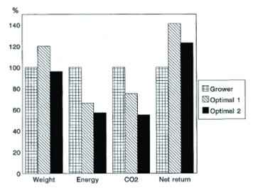
Figure 1 shows three different types of control for the crop: the first one is a traditional method of the farmer, the second one and the last one are optimal controllers. Note that two last have a better impact on energy saving, production, and total gain 19.
A dynamic optimization tool of Matlab based on optimal control theory was used to obtain time trajectories of the energy flux that minimizes total external energy input over the year while maintaining greenhouse air temperature and humidity between grower defined bounds 20,21. By giving the grower the lead in defining the bounds, the method stays as close as possible to the daily practice of its growth and experience, and no crop production models and market prices are needed.
A simulation model has been developed 22 to predict the performance of a greenhouse that is heated with a heat-pipe system. The model is validated with experimental data and is found to be in close agreement. The simulation can provide estimations of the influence of the maximum height, the heating power required in cold weather, and the heat losses from the greenhouse. In this article, no crop model is necessary.
An optimal control to regulate the open and closing of the side ventilation windows of the greenhouse can be obtained from a mathematical model such model integrates the dynamic model of the crop and the dynamic model of the greenhouse. A performance criterion was selected appropriately in order to apply the optimal control theory and obtain the trajectories that maximize the benefit of the crop and minimize the energy consumption to reach the optimal open and closing of the greenhouse windows. Through Matlab, an algorithm was built, which gives a solution for the optimal control problem, and we realized a simulation throughout a period of 5 days.
One of the main objectives is to contribute to the optimal control problem and its implementation in real-time. The tomato crop has been chosen because it is one of the most important crops in our country and is the second farm product consumed in the world. To achieve the objective, we part from the tomato and greenhouse mathematical set model considering the variable of plant and fruit dry weight, the availability of nutrients, the quantity of carbon dioxide, and the mechanism of opening and closing of the windows.
2.A dynamic model of the crop and greenhouse
Assume that a greenhouse microclimate is considered as a lumped parameter system, i.e., a greenhouse is treated as a homogeneous block (a perfectly stirred tank), which means that the inside air is well mixed. Therefore, all the heat and mass fluxes can be described per square meter. Besides crop canopy is also viewed as a big leaf. We can see that a greenhouse mainly includes the following 5 classes of variables:
The greenhouse microclimate state variables below screen: concentration
Crop growth state variables and actions: dry matter of crop WL (mg/m2), dry matter of fruit WF (mg/m2), photosynthesis rate P(mg/(sm2).
Outside climate variables: wind speed v (m/s) , etc.
Control input variables: the opening of vents to leeward
Physical parameters of material and structure: greenhouse ground area Ag (m2), greenhouse air volumeVg (m3).
The book (Economics-based Optimal Control of Greenhouse Tomato Crop Production, R.F. Tap, Thesis Wageningen Agricultural University. ISBN 90-5808-236-9. 2000. Page 31) describes the calibration and validation of the greenhouse tomato crop production model developed for optimal control purposes. The calibration of the greenhouse and crop model was performed sequentially; first, the tomato model is calibrated, and then the greenhouse model is calibrated using the outputs of the tomato model as inputs. This way, the mutual influence of the different models is partly taken into account in the calibration process were resulting in a more accurate description of the overall system behavior. Calibration parameters were chosen based on insight in the model and sensitivity analysis of the model outputs to parameter change. The calibration results were evaluated using the parameter covariance matrices and their eigenvalue decomposition. Both models were validated using independent experimental data. Calibration and validation results showed that the performance of the greenhouse model and the tomato model is comparatively reasonable to the experimental ones. Figure 2 (extracted from Tap) shows the comparison of both results for the fruit dry weight. The complete results are observed in the same Ref. 23.
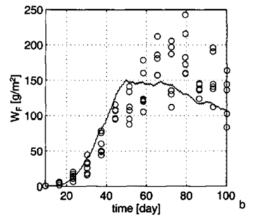
Figure 2 Results of simultaneous calibration for the fruit dry weight. replicates of measurements -simulations.
2.1.Dynamic model of the Crop
The chosen crop here as a case is tomato. This is a generative crop that poses larger challenges to the model as compared with other crops. Moreover, it is of larger economic interest. The crop model is a three-state model, with the assimilates and the fruit and leaf biomass as states. The greenhouse climate model is a relatively simple lumped parameter model, with the CO2 inner concentration as a state. It is called a big leaf-big fruit model because it makes no distinction between the number of leaves and fruits. The model works with state-space and describes the evolution of the biomass of the leaves and the fruits after the first sprout. The model in space states of the tomato crop has three principle states 19:
2.1.1.Biomass balance of nutrients
Nutrients are being produced by photosynthesis. The gross canopy photosynthesis rate in dry matter per unit area is P. Nutrients are converted to leaves and fruits; this is known as growth. Leaves and fruits have a demand for nutrients, which will be honored if there are sufficient nutrients available. We denote WB as the total nutrients in the plant, and it is expressed as dry weight per area unit. The biomass balance equation of nutrients is the following:
The biomass balance equation of nutrients ([ec13]) can take two values
depending on the nutrients abundance
where RF respiration needs of fruits,
2.1.2.Biomass balance of leaves
The leaf growth is equal to the number of nutrients converted to structural
leaf biomass in the plant, and it is given by
Depending on the abundance of nutrients
where HL is the leaf picking rate.
2.1.3.Biomass balance of fruit
Similarly to the biomass of leaf case, the growth of fruits in the plant from
the nutrients is given by
Finally, the Eq. (5) of biomass balance of fruits can take two different
values depending on nutrient abundance
2.2.Dynamic model of the greenhouse
The dynamic model of the greenhouse covers many aspects, including ground heat balance, heating system, the mass balance of water vapor and carbon dioxide, however, for this work, only the opening and closing of the side ventilation windows are considered.
2.2.1.Dynamic model of the greenhouse
The balance of carbon dioxide energy within the greenhouse is given by the equation:
The total mass of CO2 in the greenhouse is
The modeling of a greenhouse involves a large number of variables and parameters. Some of the main variables are the carbon dioxide concentration, the temperature inside the greenhouse, the water vapor mass balance, the lighting, etc.
The Eq. (7) relative to the concentration of carbon dioxide inside the greenhouse does not depend directly on the temperature or the mass balance of water vapor; however, it involves the term that controls the opening and closing of vents, the reason why this equation was chosen, in addition to simplifying the objectives of this work.
Loss of carbon dioxide mass by ventilation:
here
Carbon dioxide supply:
where:
In this greenhouse model, the position of the carbon dioxide supply valve is a control input, and it is replaced by a sinusoidal function. While uv is the flow rate of the volumetric ventilation per unit area of the greenhouse, defined by:
where pv1, pv2, pv3, pv4, and pv5 are fit parameters, to see24, v is the wind speed,
In this model, Eq. (10) relates the opening and closing of the vents, which is the control input. That is the purpose of this work.
Assuming an abundance of nutrients, the dynamic model of the crop can be represented by 3 differential equations, while the dynamic model of the microclimate is represented by one differential equation, which describes its behavior based on the energy balance of carbon dioxide.
3.General formulation of the optimal control problem
The optimal control of any system has to be based on three concepts: the dynamic model of the system, a functional and the system restrictions. In matrix notation, the equation of state is represented as follows
where x(t) is the state vector, u(t) is the control signal, and t is the time. A standard is required to help evaluate the performance of the system; normally, the function is defined by
where t0 and t
f
are the initial and final time, Φ and L are scalar functions, t
f
can be fixed or free. Starting at the initial state x(t) = x0 and
applying the control signal u(t) for
Necessary conditions for a solution. Adding the restrictions given by expression (12)
to the performance index Eq. (13) with a vector of Lagrange multipliers variants at
time
Defining the Hamiltonian Scalar Function H(x(t)), u(t), Ψ(t), t) as
By integrating the parts the Eq. (14), you get
Now consider an infinitesimal variation in u(t), δ(t). This variation produces a variation in the trajectory of the states δx(t) and a variation in the performance index δJ. This last variation can be calculated as follows
To avoid having to determine the functions δx(t) produced by δu(t), choose the
multipliers Ψ(t) such that the coefficients of δx(t) y
with the border conditions
Then δJ transforms into
If x(t0) is specified, then
this equation is called the stationary condition.
The equations of Ψ,
where u(t) is determined from the stationary condition. The conditions in the border for these differential equations are separated. This means some are defined in t = t0 and some in t = t f . x(t0)is specified by the condition,
This is a Two-Point Boundary Value Problem. Note that the state equations and the co-states are coped because u(t) depends on Ψ(t) through the stationary condition and the co-states depend on x(t) and u(t).
4.Design of the control law
Before carrying out the design of the control law, it is necessary to perform the synthesis of the control, which consists of choosing a performance index, from which it is possible to obtain a system of attached state variables. In this way, the initial and final conditions of the system are obtained. In order to perform the synthesis of the control, it is necessary to know the values of the parameters involved so that the system is close to reality, for what the substitution in Eq. (11) is performed with the values of the existing climatic conditions in the state of Puebla and Eq. (24) shows the integrated model microclimate-cultivation:
where,
and
Based on the knowledge of the problem and the requirements of the system, the following performance index is considered:
Performance index is known as the General Index for Optimum Control Systems, which includes the variables of state, the control, and scalar functions α and β, scalar functions that can be adjusted to the consideration of the designer.
The Hamiltonian scalar function is defined following the performance index, which depends on the state variables, the control input, and the new vector of Lagrange multipliers.
Therefore, the H function is as follows:
The Hamiltonian scalar function allows us to obtain a new system of differential equations, which is formed by the attached variables. Consequently, the system of attached state variables is expressed as:
To find the control vector function 𝑢(𝑡) that produces a steady value of the performance function J, the following system of differential equations must be solved:
where u(t) is determined from the stationary condition; therefore, the Hamiltonian function is partially derived concerning to the control signal, which results in:
From (32), it can be seen that the control depends on the fourth attached state
variable
5. Simulation results
In this section, we present the results of the simulation of the control law using the parameters shown in Table I. The complete system representation is:
It is not possible to use the system (6) because there are only initial conditions for the state variables, and, for the attached state variables, there are only final conditions, so it is necessary to make use of the inverse time. Once the partial derivatives in (33) have been determined,
and
where: C1 = 3.7192 x 10⁻¹¹, C2 = 1.6353 x 10⁻⁹, C3 = 4.0439 x 10⁻⁵, C4 = 1.5942 x 10⁻⁶, C5 = 0.4856 x 10⁻⁶, and C6 = 1.668 x 10⁻⁷.
It is possible to solve the system (33) and graph the behavior in the Matlab software. The behavior of the state variables, is shown in Fig. 3.
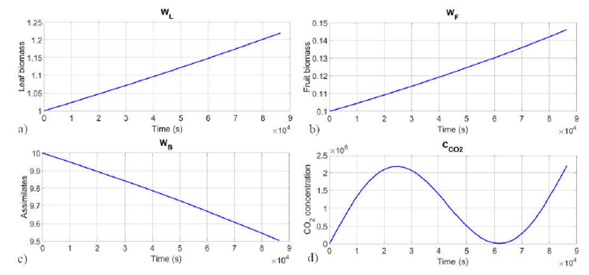
Figure 3 a) Leaf biomass behavior. b) Fruit biomass behavior. c) Assimilates behavior. d) CO2 behavior. System response.
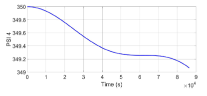
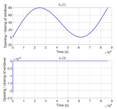
Figure 4 describes the control behavior, how a function of the fourth variable attached Ψ4; therefore, the necessary substitutions are made to convert that behavior to the function of the opening and closing of the side ventilation windows; besides it is considered that the opening to leeward and windward are done at the same time. Clearly, the selection of the mechanism to open and close the vents does not affect the structure of the validated model,
Substituting Eq. (39) into Eq. (10), we obtain that
Using Eq. (40) in Eq. (8), we obtain the following equation
In Eq. (32), it is observed that the control is in function of
The substitution of (42) in (40) is made in order to obtain
To obtain variable of interest
Table I Physical parameters related to the microclimate
| Variable | Value | Description |
| η | 0.7 | Heat absorbed in relation to the total energy of the net radiation received. |
| Vg/Ag | 3 | Reason for volume of the greenhouse per unit area. |
| 1.6637 | Concentration of carbon dioxide outside the greenhouse. | |
| pv1 | 7:17 x 10 -5 | Parameter |
| pv2 | 0:01556 | Parameter |
| pv3 | 2:71 x 10 -5 | Parameter |
| pv4 | 6:32 x10 -5 | Parameter |
| pv5 | 7:40 x 10 -5 | Parameter |
In Fig. 5, it is possible to see the 2 solutions of the quadratic equation; besides it is observed that the behavior of the first graph resembles more to the reality, reason why that result will be applied to the control system for the side ventilation windows.
6.Conclusions
This paper considered the integrated model of crop-microclimate, a situation that does not perform other research work because, generally it take into account only the model of the microclimate. The application of the theory of optimal control allowed the design of the law of control for the opening and closing of the side ventilation windows, the creation of an algorithm in Matlab solved the contour problem and allowed the simulation of the variables of state of the integrated dynamic system crop-microclimate. Although the objective of this work is not to regulate the inner optimum concentration of carbon dioxide in the greenhouse, by including such variable in the states, the optimum concentration of carbon dioxide was also obtained to the inner; therefore, the control law optimum for the opening and closing of the side ventilation windows can contribute to the regulation of this concentration. The implementation of the electronic device will provide economic benefits in saving energy consumption.

