SciELO - Scientific Electronic Library Online

 
vol.67 issue1Little group generators for Dirac neutrino one-particle statesAnalytical solution to Scholte’s secular equation for isotropic elastic media author indexsubject indexsearch form
Home Pagealphabetic serial listing  

Services on Demand

Journal

Article

Indicators

Related links

  • Have no similar articlesSimilars in SciELO

Share


Revista mexicana de física

Print version ISSN 0035-001X

Rev. mex. fis. vol.67 n.1 México Jan./Feb. 2021  Epub Jan 31, 2022

https://doi.org/10.31349/revmexfis.67.33 

Research

High Energy Physics

A new variational approach and its application to heavy quarkonia

R. Manzoora 

J. Ahmeda 

A. Rayab  c 

aCentre For High Energy Physics, Punjab University, Lahore (54590), Pakistan.

bInstituto de Física y Matemáticas, Universidad Michoacana de San Nicolás de Hidalgo. Edificio C-3, Ciudad Universitaria. C.P. 58040, Morelia, Michoacán, Mexico.

cCentro de Ciencias Exactas, Universidad del Bío-Bío, Avda. Andrés Bello 720, Casilla 447, 3800708, Chillán, Chile.


Abstract

By combining the variational principle with Heisenberg uncertainty principle in an effective Hamiltonian for heavy flavored mesons, we introduce a framework to estimate masses and radii of these states from an analytical constraint. In a novel manner, a model for quark velocity and a model for quark momentum width are introduced. These kinematical model parameters are obtained as analytical functions of inter quark separation in heavy quarkonia. The values of such quark parameters are then used in the calculation of S-wave annihilation decay rates of cc¯ and bb¯. To test the accuracy of our technique we first calculate the spin averaged masses, scalar radii and annihilation decay rates of charmonium and bottomonium without and with relativistic corrections by solving the Schrödinger wave equation with the appropriate parametrization of the Song-Lin potential. The Schrödinger wave equation is solved numerically with the matrix Numerov method and we observe a good agreement with the experimental measurements and other theoretical calculations and extract strong running coupling constant for cc¯ and bb¯ systems. In non-relativistic settings, heavy meson spectra have been obtained and extended to rather higher excited states within our framework by using bare masses of c and b quarks which we have extracted from analysis of experimental data.

Keywords: Non-relativistic potential model; charmonium and bottomonium; variational principle

PACS: 12.39.2x; 13.20.Gd; 13.25.Gv; 14.40.Gx

1.Introduction

The study of heavy quarkonia in quantum chromodynamics (QCD) is a field theoretical non-perturbative problem which has promoted the development of several techniques appropriate to address this issue. Under certain considerations, it can be simplified to a non-relativistic (NR) quantum mechanical problem by exploring the interaction strength between quarks inside hadrons in the static limit of the interaction potential (SLIP) between quarks. Lattice QCD simulations 1,2 suggest for this potential a Coulombic term at short distances plus a linearly rising part at large inter quark separations, which to-date has motivated a large number of phenomenological models (3)-(19) that capture the quantum chromodynamic traits of strong interactions. Whilst the SLIP picture for light-quarks must be taken with a grain of salt, for the case of heavy mesons, cc¯ and bb¯, this picture is accurate enough to describe the mass spectra of heavy quarkonia. Assuming spherical symmetry, the SLIP can be cast in the general form V(r)=-Ar-α+Brβ+V0, where r is the inter quark distance, A, B and V0 are constants and α and β are free parameters assessed either from Lattice QCD, see for example , or fixed by fitting the known experimental masses of hadronic states. The choice α = β =1 and V0 = 0 corresponds to the Cornell potential. The choice V0 = 0, α = 2 =β/2 corresponds to the anharmonic potential 21 and other choices give rise to commonly used potentials.

The relevant Schrödinger wave equation (SWE) with any of these SLIPs often has to be solved numerically. To that end, a vast number of numerical strategies have been implemented in literature among which, to count a few, we find the shooting method 22, the Asymptotic Iteration Method (AIM) 23 and many others such as different forms of Runge-Kutta methods. Most numerical strategies implemented for solving the SWE are as precise as going up to O(d2) of grid spacing d. The Matrix Numerov Method (MNM) (see, for instance 24) which in the context of meson physics has been put forward by the Qena group 25 and extended by our group 26, departs from a discretization of the kinetic term in the SWE in such a manner that the problem of solving the radial SWE is cast in the form of a matrix eigenvalue problem. In this form, its accuracy is of O(d6). On the other hand, many proposals of quark model (QM) potentials have used quark masses far higher than those reported in the Particle Data Booklet in various years 3-19. The quark model community has exploited the freedom in choosing quark masses (the so called constituent quark masses) and quark interaction energy (QIE) parameters in mq1+mq2+Σ=Mmeson. This hides the factual and physical values of quark masses mq1,mq2 and those of the quark interaction energy Σ.

In our present work we study the spectrum of heavy cc¯, bb¯ states. For that purpose, we use bare quark masses in SWE extracted from experimental evidence got by various Collaborations. Regarding the SLIP, we are interested in the choice of parameters α = β= 1/2 and V0 = 0, known in literature as the Song-Lin (SL) potential 27. We select this effective potential beyond the paradigmatic Cornell potential because there are a number of appealing features 28,29 that the SL potential displays better than the Cornell model. Let us recall that the SL potential has been theoretically calculated by coupling the non-Abelian character of QCD to a heavy dilaton field . From phenomenological perspective 27, the first term in this potential b/r is inspired from leptonic widths of vector mesons p, ω, Φ, J/ψ and Υ measured in experiments 31 and perturbative QCD at short distances, while the term -ar) has been motivated by considering a chromo-electric flux tube 27 between a quark Q and anti-quark Q¯ in a quarkonium system where perturbative QCD is hard to manage, and the possible colour-screening effects on strong force which are considered of considerable importance 33-36. In fact, the colour-screening in our parametrization of SL is far more simply added than in 33-36 using Cornell potential. The SL potential has been considered in 23,37,38 and applied only to low lying meson states with no or insignificant application to decay rates and other quarkonia observables. We calculate spin averaged masses of cc¯,bb¯ spectroscopic states, which are relevant for the prediction of hyperfine splittings between |1LL and |3LL states defined as 3LL - 1LL where 3LL is spin averaged mass of the triplet {3LL-1,3LL+1,3LL+3}. By considering the spin averaged wave functions at contact, we readily obtain the leptonic, diphoton, digluon, triphoton, trigluon and one photon plus 2 gluons decay rates of S-wave states by demanding agreement of 1S state for each one of these decays with the experiment. We do this to find the value of the QCD coupling constant (αs) and then use it for decay modes of 2S to 5S states. A comparison with known values of these decay widths is presented, rendering our full dynamical picture of the NR framework in fair agreement with the dynamics of these heavy meson states. We also include momentum width and velocity corrections to these decays and get their excellent agreement with experiment. We obtain wavefunctions, masses, radii, quark velocities, quark momentum widths, annihilation decay rates and strong running coupling constant for charmonium and bottomonium states in the following manner: we fit the parameters of the potential by demanding exactness of the theoretical mass of only one 1S spin averaged state of cc¯ with experimental value and then calculate all remaining spin averaged masses for heavy mesons with the parameters α = 0.7011 GeV3/2, b = 0.8912 GeV1/2 and this parametrization of SL potential makes the SWE a robust dynamical equation of heavy quarkonia even beyond the original expectations of the model 27 and extends the achievements of other similar calculations 23,37,38. We compare our findings against experimental results and other theoretical calculations and systematically extend our results up to 8S, 7P, 7D, 7F, 7G. This extension to higher states is allowed and reliable because suitable colour-screening effects are already present in confining term of our SL potential parametrization and this colour screening of the confining term in inter quark potential is seen to produce higher orbital and angular momentum excited states efficiently 33.

After preparing the firm ground from MNM we obtain the charmonium and bottomonium spin averaged masses and radii, in order to circumvent the struggle for numerical accuracy in the numerical solution, we introduce a variatonal approach combining the Heisenberg uncertainty principle and the variational principle in the Hamiltonian of the SWE. Such an approach, which we refer to simply as the variational principle (VP), imposes an algebraic transcendental relation between the masses and the radii of these states and is partially based in our previous work in 26. The results from our VP are less uncertain than those from MNM. In the remaining part of this article we present the details as follows: Section 2 introduces MNM to solve the SWE. Section 3 presents our model of the quark velocities, and the decay widths for different decay modes of spin averaged S-states of charmonia, and bottomonia. In Sec. 4 we develop a strategy of combining the variation in mesonic Hamiltonian with Heisenberg UP through our momentum width-model to establish analytical relation between spin averaged masses and radii of heavy meson states. Conclusion and further possible developments are discussed in Sec. 5. In the Appendix A to this paper we have calculated spin averaged masses by including hyperfine, spin-orbit, and tensor interactions to SL potential and compare these against the spin averaged masses in Tables I and II obtained without these spin effects while in Appendix B we have estimated the bare quark masses. The color screening is explored in Appendix C.

Table I Masses [GeV] for cc- spin-averaged S, P and D States. We calculated spin averaged masses using (∑J(2J+1)ΔJ/ ∑J(2J+1))from Ref. 62 for Cornell potential model in Refs. 27,49 for purpose of comparison with our predicted 5P and 4D spin averaged states. Inthe last column, N stands for “from Numerov Method”, E for “from Experimental mass of the meson” and VP is for “from our variationalprinciple” (Sec. 4). 

nL Exp. Masses 33 m c = 1:8 GeV (22) m c = 1:8 GeV 26 mc = 1:2 GeV [Our work] Our QIE [MeV] N/E/VP
1S 3.067 3.104 3.097 3.066 666/ 660/ 662
2S 3.649 3.703 3.673 3.764 1364/ 1250/ 1211
3S 4.040 4.090 4.017 4.208 1808/ 1640/ 1624
4S 4.415 4.375 4.276 4.545 2145/ 2015/ 1937
5S - 4.692 4.487 4.824 2424/ --/ 2194
1P 3.525 3.572 3.524 3.566 1166/ 1125/ 1042
2P - 3.986 3.907 4.055 1655/ --/ 1480
3P - 4.280 4.186 4.418 2018/ --/ 1813
4P - 4.580 4.410 4.714 2314/ --/ 2086
5P - 5.034 [27] - 4.969 2569/ --/ 2320
1D 3.769 3.806 3.791 3.902 1502/ 1369/ 1388
2D 4.159 4.185 4.090 4.292 1892/ 1759/ 1713
3D - 4.474 4.328 4.605 2205/ --/ 1991
4D - 4.898 [49] - 4.871 2471/ --/ 2231
5D - - -- 5.107 2707 --/ 2444

Table II Masses [Gev] for bb- spin-averaged S -,P -,D States. We calculated spin averaged masses using ((∑J(2J+1)ΔJ/ ∑J(2J+1)) from Ref. 62 for Cornell potential model in Ref. [48] for purpose of comparison with our predicted 5P, 4D and 5D spin averaged states. In the last column, N stands for “from Numerov Method”, E for “from Experimental mass of the meson” and VP is for “from our variational principle” (Sec. 4). 

nL Exp. Masses 33 m b = 5:2 GeV 22 m b = 5:2 GeV 26 m b = 4:668 GeV [Our work] Our QIE [MeV] N/E/VP
1S 9.444 9.473 9.460 9.444 110/ 108/ 122
2S 10.023 10.024 10.034 10.098 764/ 687/ 651
3S 10.355 10.327 10.356 10.482 1148/ 1019/ 1017
4S 10.579 10.593 10.589 10.766 1432/ 1243/ 1283
5S 10.865 10.788 10.776 10.998 1664/ 1529/ 1498
1P 9.900 9.912 9.902 9.930 596/ 564/ 496
2P 10.260 10.275 10.261 10.358 1024/ 924/ 890
3P -- 10.580 10.512 10.665 1331/ --/ 1178
4P -- 10.703 10.711 10.911 1577/ --/ 1408
5P -- 11.013 [48] - 11.119 1785/ --/ 1602
1D 10.161 10.156 10.162 10.234 900/ 825/ 810
2D -- 10.434 10.433 10.565 1231/ --/ 1093
3D -- 10.625 10.643 10.825 1491/ --/ 1328
4D -- 10.934 [48] - 11.043 1709/ --/ 1529
5D -- 11.143 [48] - 11.232 1898/ --/ 1703

2.Numerov method

The non-relativistic kinetic energy operator for a two quark system is

T=m1+m2+|p1|22m1+|p2|22m2, (1)

where m1,2 and p1,2 are the corresponding quark masses and momenta. Then the Hamiltonian of this system is

H=i=12(mi+|pi|22mi)+V(r1,r2). (2)

If these two quarks are moving in a spherically symmetric potential that depends only on their mutual separation r=|r1-r2|, namely V(r1,r2)=V(r), the problem can be decoupled into the center of mass motion of the two quark system and the relative motion of the quarks about their center of mass. Factorizing the former, the SWE for the relative motion reduces to the one-body eigenvalue problem

m1+m2+|p|22μ+V(r)Ψ(r)=ΔΨ(r), (3)

where μ=m1m2/(m1+m2) is the reduced mass of the system, Δ is the mass of the meson state and p is the momentum of quark about the center of mass of the meson. Working in spherical coordinates and separating the angular part in Eq. (3) according to Ψ(r)=Rnl(r)Ylm(θ,ϕ), where Ylm(θ,ϕ) are the spherical harmonic functions normalised to unity (with n, l and m the principal, orbital angular momentum and magnetic quantum numbers), the masses of heavy meson states are obtained by solving the radial one-body, one dimensional-like SWE ψ(r)=rRnl,

m1+m2+Σm1,m2,l,a,b;rψ(r)=Δψ(r), (4)

where we define

Σm1,m2,l,a,b;r=-12μd2dr2+l(l+1)2μr2+V(r), (5)

as an operator for QIE. In what follows, we obtain the charmonium and bottomonium spectra by solving the SWE with the SL potential 27

V(r)=-br+ar, (6)

having a and b as free parameters. We fix these parameters to the lightest cc¯ mass, and then derive the rest of the heavy quarkonium full spectrum through the Matrix Numeroved Eq. (10). Explicitly, these values are

a=0.7011 GeV32,b=0.8912 GeV12, (7)

whereas the bare quark masses are taken to be

mc=1.2 GeV,mb=4.668 GeV. (8)

In this form we parametrize charmonium mass spectrum as Δ2S+1LJ=2.4+Σ while for bottomonia we take Δ2S+1LJ = 9.334+ Σ. Our parametrization in Eq. (7) is unique and the same for cc¯ and bb¯ mesons. The masses in Eq. (8) are not arbitrary, see Appendix B for this point.

In order to solve the corresponding SWE in Eq. (4) we discretize its radial coordinate 𝑟 into N equidistant points ri separated a distance d within a preselected characteristic length rmax suitable for the description of heavy meson spectra and represent the kinetic operator in Eq. (4) in terms of the two trigonal matrices

AN,N=I-1-2I0+I1d2,BN,N=I-1+10I0+I112, (9)

such that Eq. (4) is expressed in the form as in Refs. 24-26

-12μAN,NBN,N-1ψi+VNri+ll+l2μri2+m1+m2ψi=ψi (10)

where ψi=ψ(ri) is a column matrix (ψ1,ψ2,...,ψN)T, the term in square brackets is a diagonal matrix of order N x N and I0,I-1,I+1 are respectively the square matrices of order N x N containing zeros every where except in the principle diagonal (PD), in the diagonal one step below PD, and in the diagonal one step above PD which are filled with entries as 1. Concretely, we use rmax=4 fm and fix the number of grid points with N = 350. These two numbers are obtained from the stability of the inverse of the masses of S, P and D states against variation of the number of points and the size of the domain of integration. For the sake of illustration, we show the variation of the inverse of the masses for S-states for charmonium and bottomonium with the number of grid points in Fig. 1 and with the interval of integration in Fig. 2.

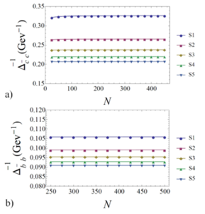
Figure 1 Stability test of the number of grid points for the prediction of the (inverse) mass of S-states for cc- and bb- at fixed rmax = 4fm. 

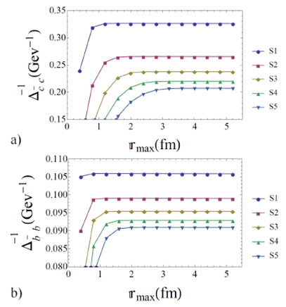
Figure 2 Stability test of the size of integration interval for the prediction of the (inverse) mass of S-states for cc- and bb- at fixed N = 350. 

2.1.Spectra

Numerical solution of Eq. (10) gives wavefunctions corresponding to spin averaged masses of charmonium and bottomonium. These are our well behaved spin averaged orthonormal wavefunctions plotted for S, P and D states in Figs. 3 and4. The spin averaged masses are shown in Tables I and II and compared against the experimental values 39 and other theoretical findings. It is important to note that finding the correct interaction energy between quarks (QIE) is a key feature for the success or failure of a quark model and is a real essence of understanding the matter in visible universe. The authors in Ref.23 and Ref.27 used charm quark mass 1.8 GeV which is 600 MeV more than our bare charm quark mass. It means that these authors estimated interaction energy 600 MeV smaller in charmonium system than ours. As for the bottom quark is concerned, these authors estimate the interaction energy to be 1066 MeV smaller when compared to ours. The correct input mass to SWE produces correct predictions and bare quark masses available so far are not less than being the correct masses of charm in Eq. (B.1) and bottom in Eq. (B.2). So our calculated interaction energies for charmonia and bottomonia must be correct in our bare quark model (BQM). A quick analysis of QIE in Tables I and II shows interaction energy in nL spin averaged states for bottomonia is smaller than that for charmonia, and QIE for (n + 1)L state is larger than for nL. As a 
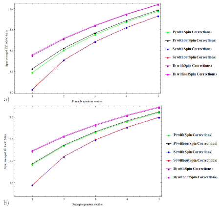
complementary note, in the Appendix A we have calculated these mass spectra by including spin-spin, spin-orbit, and tensor interactions between quark Q and antiquark Q¯ as part of the dynamical Eq. (10) instead of using the leading order perturbation method. These are the so called quarkonia mass spectra with spin effects. We have compared these spectra with those in Tables I and II obtained without incorporating the spin effects in the form of mass-plots Fig. 7.

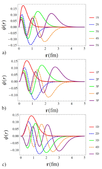
Figure 3 Wave functions for first five S-states (upper panel), P- states (mid pannel) and D-states (lower panel) of cc- mesons in the SL potential 

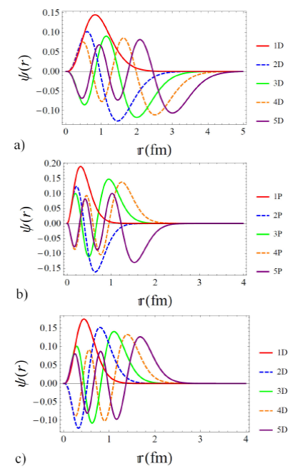
Figure 4 Wave functions for first five S-states (upper panel), P- states (mid panel) and D-states (lower panel) of bb- meson in the SL potential. 

As for the size of the bound states, the root-mean-square radii rrms can be directly obtained from the numerical solution of the SWE as,

(rrms)2=0 dr r3|Rnl(r)|2, (11)

where the symbols n and l stand for the principal and orbital angular momentum quantum number of the meson, respectively. Furthermore, the heavy quarkonia states exhibit momentum width β as function of the quarkonium size determined by their quantum numbers in our proposed functional form i

β=δrrms. (12)

Radii from Eq. (11) and momentum width from Eq. (12) for different states are reported in Table III. A variation of momentum width with the size of the S, P and D states of charmonia and bottomonia are depicted on right panels in Figs. 5 and6, along with the analytical expressions for momentum width as functions of instantaneous quark separation r. From Table III we observe that bottomonia are more compact objects than corresponding charmonia. Furthermore the charmonia sizes are roughly twice as large as those of the similar states of the bottomonia while momentum width for c-quark mesons is approximately half that of the b quark.

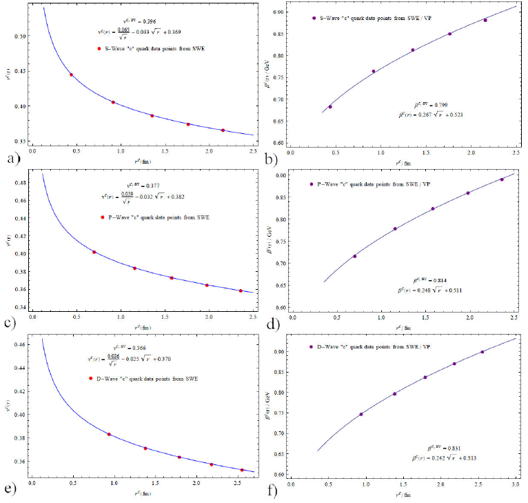
Figure 5 The velocities and momenta of charm quark within cc- versus radii of cc- obtained from SWE and our VP. 

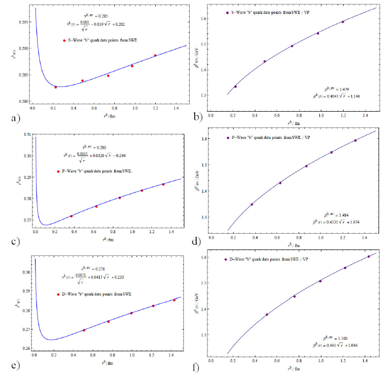
Figure 6 The velocities and momenta of bottom quark within bb- versus radii of bb- obtained from SWE and our VP. 

Table III Radii rrmscc- of cc- and rrmsbb- of b¹b states in [fm] and corresponding momentum width βcc- and βbb- in [GeV] in spin averaged S -, P- and D quarkonia states. 

nL rrmscc- (SWE)/ rrmscc-(VP)/Re. (63) βSW ECC-/βVPcc- rrmsbb- (SW E/ rrmsbb-(VP)/Ref.(64) βSW Ebb- βVPbb-
2S 0.915/ 0.922/ 0.91 0.765/ 0.760 0.488/ 0.501/ 0.545 1.434/ 1.397
3S 1.352/ 1.363/ 1.38 0.813/ 0.810 0.737/ 0.755/ 0.805 1.493/ 1.457
4S 1.762/ 1.773/ 1.87 0.851/ 0.846 0.972/ 0.991/ 1.030 1.544/ 1.514
5S 2.151/ 2.161/ 2.39 0.882/ 0.879 1.200/ 1.216/ 1.232 1.588/ 1.562
1P 0.697/ 0.775/ 0.71 0.717/ 0.645 0.370/ 0.416/ 0.435 1.350/ 1.202
2P 1.155/ 1.195/ 1.19 0.779/ 0.753 0.628/ 0.658/ 0.711 1.432/ 1.368
3P 1.577/ 1.601/ 1.67 0.824/ 0.812 0.869/ 0.893/ 0.945 1.496/ 1.456
4P 1.976/ 1.992/ - 0.860/ 0.853 1.097/ 1.118/ 1.154 1.549/ 1.521
5P 2.343/ 2.367/ - 0.891/ 0.887 1.317/ 1.336/ 1.346 1.594/ 1.572
1D 0.936/ 1.097/ 0.96 0.748/ 0.638 0.507/ 0.601/ 0.593 1.379/ 1.165
2D 1.380/ 1.472/ 1.44 0.797/ 0.747 0.760/ 0.818/ - 1.448/ 1.345
3D 1.791/ 1.850/ 1.94 0.838/ 0.811 0.994/ 1.036/ - 1.508/ 1.448
4D 2.178/ 2.220/ - 0.871/ 0.856 1.218/ 1.251/ - 1.559/ 1.560
5D 2.497 /2.581/ - 0.900/ 0.891 1.434/ 1.460/ - 1.604/ 1.575

3.Other quarkonia observables

From the discussion of the previous section, we obtain a few parameters that allow us to characterize the dynamics of these heavy quark systems.

3.1.A model for quark velocities

Quark velocity is a vital ingredient in taking a decision whether to describe quark dynamics in QCD perturbatively or non-perturbatively, and in the determination of hadron masses using string quark model Ref.46. The root-mean-square velocity of bottom quark in the bb¯ ground state is about 0.3𝑐 and that of the charm quark in the lowest energy state of the cc¯ is 0.5c (where c is the speed of light in vacuum; see, for instance, Ref.47). Moreover, and speaking naively, in the study of various types of decays of a hadron the distribution of angular momentum-momentum of the partons within it among possible decay products is a necessary item both in experimental measurements (for example the JPC of a meson) and in theoretical calculations of decays (as we do in Subsec. 3.2.1 in the form of momentum width and velocity corrections). Incidentally, how the momentum is distributed among constituents is equally important for inelastic scattering of leptons from composite particles as in deep inelastic scattering experiments. This concept is of prime importance for explanation of the, effect observed by the European Muon Collaboration (EMC) , the EMC effect, where in Deep Inelastic Scattering (DIS) experiments the scattering cross-section of leptons from quarks in nucleons of heavy atomic nuclei is smaller than their scattering cross-section from quarks in nucleons of light atomic nuclei. In addition, this momentum distribution is fundamentally dependent on parton velocity, see for example Eqs. (69), (70) and (106) in Ref. for a flux tube quark model. For these reasons, we introduce a model for the quark velocity which is applicable not only for the ground states of hadrons, but also for excited states. Another reason for promulgating this definition is of direct use for SWE and for the variational approach which we describe below, in Sec. 4. The quark velocities in states other than the ground state of quarkonia have never been reported as far as we know. We propose two ways for calculating the quark velocity, a first parametrization is motivated from simple dimensional analysis and the idea that two particles are revolving around their common center of mass as if no QCD glue or some other medium is present between and around the two particles. The explicit parametrization is

vF=βmQ, (13)

where β is the quark momentum found from Eq. (12), mQ is the bare quark mass. A second parametrization is based on our model that whatever is present in the meson in addition to quarks half of the meson mass should come from one quark and its dressing. In other words, the quark has to drag along it the field it is moving in. So we assume its inertia as half of the meson mass and thus we introduce

vS=2βΔ, (14)

where Δ is the QQ¯ meson mass. This definition can be extended to the case of baryons, composed entirely of heavy quarks, the effective quark inertia would be one third the mass of that baryon and we shall get a factor of three in Eq. (14) in place of a factor of two. In our view, Eq. (14) should be more realistic because, a priori, it takes into account whatever is present in the meson along with the quarks and Eq. (13) should be a special case of our model given by Eq. (14) in the limit where QIE is negligible as compared to sum of the bare quark masses. Thus, we adhere to Eq. (14) and report quark velocities in S, P and D spin averaged states of heavy quarkonia in Tables IV andV, which are in fair agreement with the overall assessment reported in Ref.47. These quark velocities would be of essential importance for determining inclusive decay rates by using Eqs. (27) and (33) of Ref. and the references therein, for all spectroscopic states of heavy quarkonia instead of the Bc(1S-wave) only.

Table IV Velocities from SWE and our VP (Sec. 4) in natural units, of the charm quark in orbitally and radially excited states of charmonium. 

States (n) S P D
vF vS,SW E/vS,V P vF vS,SW E/vS,V P vF vS,SW E/vS,V P
1 0.59 0.445/0.453 0.60 0.402/0.375 0.62 0.383/0.337
2 0.64 0.406/0.420 0.65 0.384/0.388 0.66 0.371/0.363
3 0.68 0.386/0.401 0.69 0.373/0.385 0.70 0.364/0.369
4 0.71 0.374/0.390 0.72 0.365/0.380 0.73 0.357/0.370
5 0.74 0.366/0.383 0.74 0.358/0.376 0.75 0.353/0.368

Table V Velocities from SWE and our VP (Sec. 4) in natural units, of the bottom quark in orbitally and radially excited states of bottomonium. 

States(n) S P D
vF vS,SW E/vS,V P vF vS,SW E/vS,V P vF vS,SW E/vS,V P
1 0.286 0.283/0.289 0.289 0.272/0.244 0.295 0.270/0.229
2 0.307 0.284/0.280 0.306 0.276/0.268 0.310 0.274/0.258
3 0.319 0.285/0.282 0.321 0.281/0.277 0.323 0.279/0.271
4 0.331 0.287/0.285 0.332 0.284/0.283 0.334 0.282/0.280
5 0.340 0.289/0.288 0.342 0.287/0.287 0.344 0.286/0.285

We plot quark velocities versus radii of mesons in their different quantum states in Figs. 5 and6. We observe that for cc¯ and bb¯, the velocities of charm and bottom quarks in S, P and D states follow a universal rule,

vS(r)=σr+εr+vS0, (15)

while the momentum widths behave as

β(r)=ρr+β0, (16)

where σ(fm), ε(fm(-1/2)), vS0, ρ(GeVfm(-1/2)) and β0(GeV) depend upon the principal- and orbital angular momentum-quantum numbers of the quarkonium state. An interesting conclusion that we reach at by comparing Tables IV andV is that velocities of charm and bottom quarks predicted by Eqs. (13) and (14) do not differ significantly for low lying mesons but this difference becomes conspicuous for higher quarkonia states. In fact, the difference in predictions for bottom quark in Table V is almost negligible. The latter means that as per our velocity model, the heavier quarksare surrounded by a little amount of fields contributing to the the mass of meson via QIE and vice versa, but as the heavier quarks get apart as in D-wave bottomonia, predictions start differing. This observation is also supported by comparing the QIE’s of (nL)cc¯ with (nL)bb¯ in Tables I andII. It is not without interest when we compare our quark-velocity Tables IV andV with quark-velocity Table I of Ref.46. It has also been measured in experiments (see Ref.48,50) that first generation quarks in heavier atoms have velocities 10 to 20% smaller than their velocities in lighter atoms. This trend of EMC effect Ref. 48,50 is predicted by our velocity model Eq. (14) as we look horizontally from left to right the direction of increasing mass of mesonic QQ¯ atoms in Table IV for the second generation charm quark, and from left to right in Table V for the third generation bottom quark, and this is a practical success of our model of quark velocities. We state these findings as follows: quark velocity decreases due to an increase in its interaction energy with other quark, and this interaction energy is larger as the interquark separation grows bigger. Due to increase in both of the interaction energy and interquark separation, the mass of the bound state of quarks rises (compare for example 1Scc¯ with 1Pcc¯ with 1Dcc¯). Hence, quarks move at slow velocities in heavier bound states and vice versa.

3.2.Annihilation decay rates

To further strengthen our use of bare quark masses in the non-relativistic potential model and the claimed improved accuracy of the Matrix Numerov method, we have opted to calculate the various decay rates of spin averaged S-wave charmonia and bottomonia. Contrary to the general practice of proposing Gaussian, or hydrogenic functions with one or two free parameters, we have calculated the wave functions for the spin averaged quarkonia as solutions of SWE. The leptonic (e+e-) -, diphoton (γγ) -, digluon , triphoton (γγγ), trigluon (ggg) -, and 1 photon-2 gluon decays are of pivotal importance in identifying and producing the resonances. These decays are also helpful for establishing the conventional mesons and other multi-quark structures Refs.51,52. The decay rates of S-wave quarkonia are 53-55

Γ(nSe-e+)=|Rns(0)|2Δns24eQ2α21-16αs3π, (17)

ΓnS3g=Rns(0)2mQ210π2-981παs3×1-4.9αsπ (18)

ΓnSγγγ=Rns(0)2mQ24π2-93πeQ6α3×1-12.6αsπ (19)

ΓnSγgg=Rns(0)2mQ28π2-99πααs2eQ2×1-6.7αsπ (20)

Γ(nSgg)=|Rns(0)|2mQ22αs23,1+4.8αsπ, (21)

Γ(nSγγ)=|Rns(0)|2mQ23eQ4α211-3.4απ, (22)

where Rns(0) is the meson wave functions at contact, which we take from our numerical solutions of Eq. (10), Δns the mass corresponding to the meson state, mQ the bare quark mass, eQ the quark electric charge in elementary units e, α=e2/(4π) the fine structure constant and αs is the strong coupling constant. In each of the above expressions for decay rates, the last factor in parentheses comes from the one-loop radiative QCD corrections. It is important to mention that value of αs is not available in the two free parameters of SL potential, see Ref.23,27 and Eq. (7). Thus, to move forward, we fit the experimentally known one value of the decay rate of each channel from Eqs. (12) to (22) in the 1S state and extract the value of αs for that decay rate. Then we produce all remaining values for 2S, 3S and so on states for each channel. The values extracted for αs pertaining to decay modes in Eqs. (17) to (22) are displayed in Table VI for charmonia and bottomonia. The over all average value of αs for QQ¯ comes out to be 0.3515 ± 0.761.

A comprehensive review about the strong running coupling constant αs within the effective potential approach is given in section 4.3 of the Ref.56. Our values of the strong coupling constant are in agreement with the findings of that work.

Annihilation decay rates are reported in Tables VII toXVIII along with a comparison against experimental results and other theoretical calculations where available.

Table VI The strong running coupling α s  

Quarkonia(nS) Γe+e- Γ ggg Γ γγγ Γ γgg Γ gg Γ γγ αsαv
cc- 0.0147 0.1834 0.1948 0.2244 0.2780 0.5435 0.2872±0.1328
bb- 0.4268 0.2091 0.2475 0.0943 0.2968 0.7771 0.4058±0.1946

Table VII Leptonic decay widths [keV] of spin averaged S-wave cc- states 

State Our Γ(nS)/Γc(nS) Exp. [38] [39] [40] (Γ (nS−> e + e - ) / Γ 1S->e + e - ) our/Exp. [26]
1S 5.55 5.55 5.63 3.112 1.00/1.00
2S 2.18 2.33 2.19 2.197 0.39/(0.45±0.08)
3S 1.34/0.91 0.86 1.20 1.701 0.16/(0.16±0.04)
4S 0.97/0.63 0.58 0.63 - 0.11/(0.11±0.04)
5S 0.76/0.47 - 0.24 - 0.08/-

Table VIII Three-gluon decay widths [keV] of spin averaged S-wave cc- states 

State Our Γ(nS)/Γc(nS) Exp. [38] [41] [42] (Γ (nS−> ggg)/Γ (1S− > ggg)) our/Exp.
1S 59.45 59.55 269.06 52.8±5 1.00/1.00
2S 35.26/30.48 31.38 112.03 23±2.6 0.51/0.53
3S 27.14/23.52 - 94.57 - 0.40/-
4S 22.85/19.85 - 88.44 - 0.33/-
5S 20.12/17.38 - 85.30 - 0.29/-

Table IX Three-photon decay widths [eV] of spin averaged S-wave c c- states 

State Our Γ(nS)/Γc(nS) Exp. [38] [41] (Γ (nS− > γγγ)/Γ (1S− > γγγ)) our/Exp.
1S 1.08 1.08±0.032 3.95 1.00/1.00
2S 0.64/0.45 - 1.64 0.42/-
3S 0.49/0.33 - 1.39 0.31/-
4S 0.42/0.27 - 1.30 0.25/-
5S 0.37/0.23 - 1.25 0.21/-

Table X Two-photon decay widths [keV] of spin averaged S-wave c c- states 

State Our Γ(nS)/Γ c (nS) Exp. [38] [40] [41] (Γ (nS− > γγ)/Γ (1S− > γγ)) our/Exp.
1S 5.10 5.1±0.4 6.96 6.62 1.00/1.00
2S 3.02/2.12 2.15±0.6 10.45 2.88 0.42/0.42
3S 2.33/1.58 - 1.03 2.44 0.31/-
4S 1.96/1.28 - - 2.30 0.25/-
5S 1.73/1.09 - - 2.21 0.21/-

Table XI Two-gluon decay widths [MeV] of spin averaged S-wave cc- states 

State Our Γ(nS)/Γ c (nS) Exp. [38] [44] [45] (Γ (nS− > gg)/Γ (1S− > gg)) our/Exp.
1S 28.64 28.6±2.2 13.07 15.70 1.00/1.00
2S 16.99/10.05 14±7 9.53 8.10 0.35/(0.49±0.28)
3S 13.08/7.51 - 4.41 - 0.26/-
4S 11.01/6.16 - - - 0.22/-
5S 9.71/5.22 - - - 0.18/-

Table XII (One-photon,two-gluon) decay widths [keV] of spin averaged S-wave cc- states 

State Our Γ(nS)/Γ c (nS) Exp. [38] [41] (Γ (nS− > γgg)/Γ (1S− > γgg)) our/Exp.
1S 8.18 8.18±0.25 9.00 1.00/1.00
2S 4.85/2.87 2.93±0.16 3.75 0.35/0.36
3S 3.73/2.14 - 3.16 0.26/-
4S 3.14/1.76 - 2.96 0.22/-
5S 2.77/1.49 - 2.85 0.18/-

Table XIII Leptonic decay widths [keV] of spin averaged S-wave b b- states 

State Our Γ(nS) Exp. [38] [46] [47] (Γ nS− > e+e− /Γ 1S− > e+e− )
1S 1.336 1.34±0.018 0.998 1.60 1.00/1.00
2S 0.610 0.612±0.011 0.439 0.64 0.46/0.46
3S 0.412 0.443±0.008 0.341 0.44 0.31/0.33
4S 0.318 0.322±0.041* 0.298 0.35 0.24/0.24
5S 0.262 0.310±0.070 0.265 0.29 0.20/0.23

*This decay width is not correct in Table (XVII) of the Ref. 59

Table XIV Three-gluon decay widths [keV] of spin averaged S-wave b b- states 

State Our Γ(nS)/Γ c (nS) Exp. [38] [59] [58] (Γ (nS− > ggg)/Γ (1S− > ggg)) our/Exp.
1S 44.14 44.13±1.09 50.8 47.6 1.00/1.00
2S 23.05/17.44 18.8±1.59 28.4 26.3 0.40/(0.43±0.04)
3S 16.78/12.36 7.25±0.85 21 19.8 0.28/0.16
4S 13.67/9.82 - 16.7 15.1 0.22/-
5S 11.77/8.26 - 14.2 13.1 0.18/-

Table XV Three-photon decay widths [keV] of spin averaged S-wave bb- states 

State Our Γ(nS)/Γ c (nS) Exp. [38] [59] [58] (Γ (nS− > γγγ)/Γ (1S− > γγγ)) our/Exp.
1S 1.95 x 10⁻⁵/1.54 x 10-5 - 1.94 x 10⁻⁵ 1.7 x 10⁻⁵ 1.00/1.00
2S 1.02 x 10⁻⁵ /7.72 x 10-6 - 1.09 x 10⁻⁵ 9.8 x 10⁻⁶ 0.50/-
3S 7.43 x 10⁻⁶ /5.48 x 10-6 - 8.04 x 10⁻⁶ 7.6 x 10⁻⁶ 0.36/-
4S 6.05 x 10⁻⁶ /4.35 x 10-6 - 6.36 x 10⁻⁶ 6.0 x 10⁻⁶ 0.28/-
5S 5.21 x 10⁻⁶ /3.66 x 10-6 - 5.43 x 10⁻⁶ 0.24/-

Table XVI Two photon decay widths [keV] of spin averaged S-wave bb- states 

State Our Γ(nS)/Γc(nS) Exp. [38] [59] [58] (Γ (nS− > γγ)/Γ (1S− > γγ)) our/Exp.
1S 1.05/0.83 - 1.05 0.94 1.00/1.00
2S 0.55/0.42 - 0.489 0.41 0.51/-
3S 0.40/0.29 - 0.323 0.29 0.35/-
4S 0.32/0.23 - 0.237 0.20 0.28/-
5S 0.28/0.20 - - - 0.24/-

Table XVII Two gluon decay widths [keV] of spin averaged S-wave b b- states 

State Our Γ(nS)/Γc(nS) Exp. [38] [59] [58] (Γ (nS− > gg)/Γ (1S− > gg)) our/Exp.
1S 17.90/14.08 - 17.9 16.6 1.00/1.00
2S 9.35/7.07 - 8.33 7.2 0.50/-
3S 6.80/5.01 - 5.51 4.9 0.36/-
4S 5.54/3.98 - 4.03 3.4 0.28/-
5S 4.77/3.35 - - - 0.24/-

Table XVIII One photon-Two gluon decay widths [keV] of spin averaged S-wave bb- states 

State Our Γ(nS)/Γc(nS) Exp. [38] [59] [58] (Γ (nS− > γgg)/Γ (1S− > γgg)) our/Exp.
1S 1.19 1.19 ± 0.33 1.32 1.2 1.00/1.00
2S 0.62 0.612 ± 0.011 0.739 0.68 0.52/0.51
3S 0.45/0.23 0.20 ± 0.04 0.547 0.52 0.19/0.17
4S 0.37/0.18 - 0.433 0.40 0.15/-
5S 0.32/0.15 - 0.370 - 0.13/-

3.2.1.The Velocity and Momentum Width Corrections In Annihilation decay rates

Most NR quark model calculations usually fail to produce decay rates agreeable with experiment. The root of this failure lies in the absence of proper account of velocities and momentum widths of the two valence quarks going to annihilate each other in a meson. We have found the momentum correction factor

Λpc=1-βcc¯mc2, (23)

in charmonia annihilation decays except for the decays to three gluons, where this factor is,

Λpcggg=1-βcc¯2mc2. (24)

The momentum width correction factor in all bottomonia annihilation decays is

Λpb=1-2βbb¯mb2. (25)

The velocity correction factor for all charmonia annihilation decays is

Λvc=1-vSc2, (26)

and this velocity factor in the case of bottomonia annihilation decay rates happens to be

Λvb=1-vSb2, (27)

except for annihilation to γgg for which the velocity correction factor is

Λvbγgg=1-2vSb, (28)

where vSc and vSb are, respectively, the velocities of c and b quarks from our velocity model in Eq. (14). For the case of quarkonia annihilations, the overall correction factor is ΛpQΛvQ to be multiplied with expressions in Eqs. (17) to (22) while Q is either c or b quark. The corrected decay rates denoted by Γc are reported in Tables VII toXVIII. The inclusion of momentum width and velocity corrections give decay rates in agreement with experiment and this is another validation about the correctness of our velocity model, Eq. ([jam2]), and the momentum width model, Eq. (14). The ratio Γ(nS)/Γ(1S) for n > 1 is seen to remain always less than 0.55 and more than 0.05. Equations (23) to (28) impose very tight constraints on the allowed momentum widths and velocities of heavy quarks while they are in a quarkonium. This is so because any change in the exponents or in the multiplication factor of velocity or momentum spoils the consistency of theoretical decay rates with experiment.

4.A Variational Approach

A subtle combination of the Heisenberg uncertainty Principle and the variation of mesonic Hamiltonian can be used to estimate the masses of charmonium and bottomonium as follows. The radial Eq. (4) can be written as,

m1+m2-12μ1rd2dr2r+ll+12μr2+V(r)×Rnlr=Rnl(r) (29)

This means radial Hamiltonian becomes (because radial component of momentum operator is p^r=-i[1r][r]r),

HR=m1+m2+pr22μ+l(l+1)2μr2+V(r). (30)

We have modeled the quark momentum of this equation in a peculiar way which is described next.

We define symmetric point as the one for which all three cartesian components of any 3-vector are equal in magnitude. This means in cartesian space,

r=3x, (31)

prβ=3βx. (32)

This definition turns Eq. (30) into the following effective Hamiltonian:

HR=m1+m2+32μβx2+l(l+1)6μx2+V(3x). (33)

Here we invoke the Heisenberg uncertainty Principle,

ΔxΔpx12, (34)

as follows: A little cerebration reveals that the equality sign in Eq. (34) would hold for ideal systems (for which experimental as well as theoretical uncertainties are frozen at the minimum possible values of Δx and Δpx), while the inequality sign in Eq. (34) would come when the system experiences all sorts of “dissipative and interactive" effects. From Tables II andIII, we observe that even in the lowest 1S state the QIE is not zero, which means QQ¯ system always has medium in which quarks move. Therefore, the equality sign in Eq. (34) cannot hold. With these key ideas on board, we parametrize the uncertainty relation in the form (that will become clear below)

ΔxΔpx=δ3, (35)

where δ is real, positive number more than one and we define it as,

δ2n-1+l+3δn.(1-l)+2n-1+l+321-δn,(1-l), (36)

where δn,1-l is the Kronecker delta. This definition is in accordance with the momentum width of known botommonium and charmonium states (see, for instance, Refs. 25,26,67) and is convenient for the discussion below, as we shorty explain. By keeping in mind the quantum indeterminacy in position and momentum of quark in a meson, let us define the notation in which Δx is x¯ -the mean of the position co-ordinate of quark relative to center of mass of the meson, and similarly Δpx by the mean quark momentum width β¯x about center of mass. With these definitions, whatever physical quantity A we calculate in our VP corresponds to the average A of many measurements of a and in essence the same as expectation value of a Hermitian operator A^ from some linear vector space acting on a Hilbert space of states the meson could be in.

Thus, from Eq. (35),

β¯x=δ3x¯. (37)

The use of Eq. (31) and Eq. (32) gives,

β¯=δr¯, (38)

and, in our notation, Eq. (33) becomes

H¯R=m1+m2+32μβ¯x2+l(l+1)6μx¯2+V(3x¯). (39)

Now we use this expression for computing meson radii and masses in the follwing way. Equation (37) makes Eq. (39) altogether a function of one variable x¯ only,

H¯R(x¯)=(m1+m2)+δ2+l(l+1)6μ1x2¯+V(3x¯). (40)

This is the Hamiltonian of our meson system QQ¯ that depends on x¯, which we regard as a variational parameter. Thus, minimizing H¯R with respect to x¯, we reach to the constraint

-δ2+l(l+1)3μ1x¯3+V(3x¯)x¯=0. (41)

Its solution gives x¯=xmin, and when this value is substituted in Eq. (40) then we identify H¯R(xmin) as the mass of the meson denoted by ΔVP written as,

VP=m1+m2+δ2+l(l+1)6μ1xmin2+V3xmin (42)

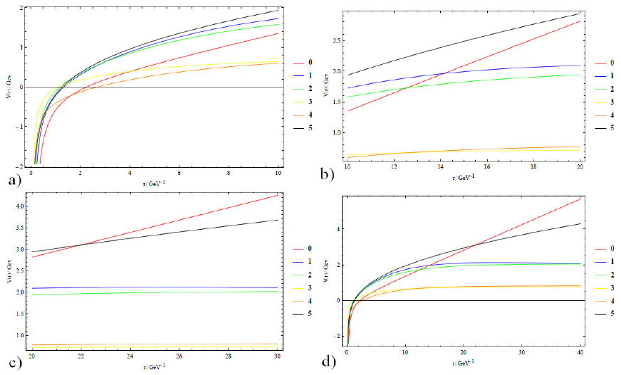
Let us apply this general procedure to a concrete example in which SLIP is the Song-Lin potential,

V(r¯)=-br¯+ar¯. (43)

Upon inserting this potential into Eq. (40), we reach at the transcendental relation

(3)54μay5+(3)34μby3-2(δ2+l2+l)=0, (44)

where y=x¯. Equation (44) has only one real root for which H¯R(x¯) is minimum and which we denote as ymin. All other four roots are complex and hence discarded being extraneous. Thus solution of quintic equation gives,

x¯=xmin=ymin2. (45)

Equation (45) used in Eq.(31) with our SL parametrization Eqs. (7) and (8) give the radii of cc¯ and bb¯ mesons reported in Table III along with root mean square radii obtained from SWE using Eq. (11) and compared with Refs.44,45. The agreement of our VP with SWE for quarkonia radii is excellent.

Substitution of the root Eq. (45) in Eq. (52) produces the meson mass,

VP=m1+m2+δ2+l(l+1)6μ1xmin2-b3xmin+α3xmin (46)

The ground state mass formula is

VP(1S)=m1+m2+12μ12xmin2-b3xmin+α3xmin (47)

and the higher states have the mass formula,

VP(nL)=m1+m2+δ2+l(l+1)6μ12xmin2-b3xmin+α3xmin (48)

The masses of cc¯ and bb¯ mesons from Eqs. (47) and (48) are reported in Table XXIII and compared with experimental values as well as those from SWE. Again the agreement of masses from our VP with experiment and SWE is remarkable. It is further emphasized that mass values from our VP are closer to experimental findings than those predicted by SWE through MNM. It implies our VP is more accurate than MNM. We also compare our VP masses of S-, D-, F- and G-waves with sophisticated calculations of Refs. in Tables XIX toXXII. The SWE is found not accurate enough in predicting higher quarkonia masses, but Tables XIX toXXIII show our VP works better not only for low lying states but it is very much suitable for spectroscopy of higher quarkonia states as well.

Table XIX Masses (in [GeV ]) of higher S wave heavy quarkonia from our VP compared with those from Screened Cornell potential (SP), Refs. 59. Here, N is for “from Numerov method”. 

Quarkonia 6S 7S 8S 9S 10S
cc-NVP/(D.Ebert, Nosh) 5.066/4.817/(5.164,4.973) 5.281/5.014/- 5.478/5.192/- 5.673/5.356/- 5.890/5.508/-
bb-NVP/SP 11.196/11.017/10.998 11.370/11.178/11.155 11.527/11.323/11.294 11.671/11.454 /- 11.804/11.576/-

Table XX Masses (in [GeV ]) of D-wave heavy quarkonia from our VP compared with those from Bethe-Salpeter equation, Ref. 60

Quarkonia 1D 2D 3D 4S 5S 6D 7D
cc-VP/SB 3.789 /3.820 4.113/4.151 4.391 /4.405 4.631/4.611 4.844/4.781 5.035/- 5.20/-
bb-VP/SP 10.146/10.15 10.429 /10.45 10.664/10.70 10.865 /10.90 11.039 /11.08 11.195/- 11.336/-

There are some more add ons from our VP. We use Eq. (45) in Eq. (31) and then result in Eq. (37) to get βVPcc¯ and βVPbb¯, which are reported in Table III. We use Eqs. (38), (47) and (48) in Eq. (14) to get vS,VP for different states of heavy quarkonia reported in Table IV. The quantity within parentheses in Eqs. (47) and (48) is the QIE which we report in Tables I andII. So every thing done by SWE numerically is more accurately and efficiently done analytically by our quantum mechanical VP.

5.Conclusion

In this article, we have explored the mass spectra of charmonia and bottomonia in a non-relativistic framework invoking the Song-Lin potential as the effective interaction that binds heavy quarks in these meson systems with a single set of parameters. By numerically solving the resulting SWE through the Numerov strategy, we were able to calculate spin averaged masses of S, P, D, F and G states. For the sake of illustration, we have not included in the discussion the techniques and ideas of spin or tensor interactions. These findings are straightforwardly extended in the Appendix A.

We have calculated S-wave annihilation decay rates without and with momentum width and velocity corrections by using wave functions at contact obtained from MNM. The agreement of theory with experiments after applying the corrections indicate that expressions for these decay rates should be revisited by properly incorporating the quark velocities and momentum widths so that the factor |ψ(r=0)|2 of wave function at contact gets replaced with |ψ(r=0,v,β)|2. This factor may be calculated by identifying the string fragmentation in the Lund Model with decay of a meson and using our VP based momentum Eq. (16) as transverse momentum distribution in the Lund Area Law. The linear rise in scalar part of the Cornell potential is inappropriate for calculation of higher excited states of mesons unless other contributions like the readjustments of the constituent quark mass, the free parameters in SLIPS and the complicated relativistic corrections in heavy quarkonia are added. The remedy to this issue has been sought in the color screening of SLIPS (see Appendix C).

The quark kinetic energies found from Table III using μv2/2 and β2/(2μ) where μ is the reduced mass of two bare quarks, are in good agreement with each other. This establishes the validity of our models of quark- velocities and momentum widths. The EMC effect observed in atomic nuclei for first generation quarks is correctly predicted by our quark velocity model in the mesons for second generation c quark and third generation b quark respectively in cc¯ and bb¯. It would be interesting to calculate these velocities in the Bc meson which should be such that velocity of c quark in Bc is less than that in cc¯ and the velocity of b quark in Bc is more than that in bb¯. This would complete the theoretical testing of EMC effect in heavy quarkonia. From Tables IV andV it is observed that vF is about (1.3 - 2)vS for c quark and vS is approximately vF for b quark. So we conclude our velocity model is more general than the usual velocity Eq. (13) which becomes a special case of our model, Eq. (14). From the analytical expressions of quark velocity in Eq. (15) and momentum width (16) and the spatial rates of changes (the gradients) their of, the result is: c quark velocity decreases with increasing quark separation but at the same time quark momentum width increases. This is an indication that QIE causes an increase in the constituent mass of quark in the form of so-called quark dressing and, as for the b quark velocity is concerned, it increases with increasing interquark separations but the increase in the b quark momentum width is seen to be more than this, which leads to increase in constituent mass of b quark like the c quark. This is one of the main reasons for which the eigenvalues of SWE with any one fixed value of the constituent quark mass as in Refs. 3-18 spoils the accuracy of the calculation for mesons in higher excited states. This unpleasant feature is -to some extent- also visible in Table XIX with the MNM, but it is absent in our VP mass spectra. It is the landmark of our VP, and we find it more convenient the use of constituent quark masses in quark model calculations. Coming back to gradients, all of them are observed to decrease such that change in velocity of c quark occurs opposite to the direction in which c quark momentum changes and this happens in the same direction for the case of b quark. This is one of the reasons that QIE is more in cc¯ than in bb¯. Finally, our VP loses its accuracy nowhere in the mass spectrum when we compare its predictions against other techniques as observed from Tables XIX toXXIII. As far as meson wave functions are concerned, these can be obtained by using Virial Theorem as in Ref. 73. This makes our VP a robust dynamical method applicable to any two-body non relativistic bound state held together by a suitable interaction potential V(r).

Table XXI Masses (in [GeV]) of F -waves heavy quarkonia from our VP compared with those from Screened Cornell potential (SP) Refs. 60

Quarkonia 1F 2F 3F 4F 5F 6F 7F
CC-VPD.Ebert 4.056/4.071 4.3182 /4.406 4.556 /- 4.770/- 4.964 /- 5.141/- 5.3052 /-
bb-V P/SP 10.380 /10.366 10.603/10.609 10.802/10.812 10.979 /10.988 11.138 /- 11.281 /- 11.4135/-

Table XXII Masses (in [GeV]) of G-wave heavy quarkonia from our VP compared with those from Screened Cornel potential (SP) Refs. 59 and D. Ebert 61

Quarkonia 1G 2G 3G 4G 5G 6G 7G
CC-VPD.Ebert 4.2783/4.345 4.5008 /- 4.7095 /- 4.9023/- 5.0804 /- 5.2457/- 5.4000 /-
bb-V P/SP 10.570/10.534 10.756/10.747 10.929/10.929 11.087 /- 11.232 /- 11.366/- 11.490/-

Table XXIII Masses [GeV] for c c- and b b- spin-averaged S, P and D states from our VP compared with those from SWE and from the experiments. 

nL Expcc-. [33] (Numerov) cc- Our VP Exp bb- . [33] (Numerov)bb- Our VP
1S 3.067 3.066 3.062 9.444 9.444 9.458
2S 3.649 3.764 3.611 10.023 10.098 9.987
3S 4.040 4.208 4.024 10.355 10.482 10.353
4S 4.415 4.545 4.337 10.597 10.766 10.619
5S 4.487 [26] 4.824 4.595 10.865 10.998 10.834
1P 3.525 3.566 3.442 9.900 9.930 9.832
2P 3.907 [26] 4.055 3.879 10.260 10.358 10.226
3P 4.186 [26] 4.418 4.213 10.512 [57] 10.665 10.514
4P 4.409 [26] 4.714 4.486 10.711 [57] 10.911 10.744
5P 4.807 4.969 4.720 10.014 11.119 10.938
1D 3.769 3.902 3.788 10.161 10.234 10.146
2D 4.159 4.292 4.113 10.432 [57] 10.565 10.429
3D 4.328 [26] 4.605 4.391 10.643 [57] 10.825 10.664
4D 4.520 4.871 4.631 11.011 11.043 10.865
5D 4.885 5.107 4.844 11.389 11.232 11.039

Acknowledgements

RM thanks Higher Education Commission of Pakistan for providing funds to complete this project. AR acknowledges valuable discussions with K. Raya.

References

1. A. Bazavov et al. for the HotQCD Collaboration, Phys. Rev. D 90 (2014) 094503. https://doi.org/10.1103/PhysRevD.90.094503 [ Links ]

2. M. A. Escobedo, Effective Field Theory and Lattice QCD approaches for hard probes in QCD matter Proceedings of the International Conference on Hard and Electromagnetic Probes of High-Energy Nuclear Collisions, 2018. Preprint: arXiv:1812.06344. [ Links ]

3. S. Godfrey and K. Moats, Bottomonium mesons and strategies for their observation. Phys. Rev. D 92 (2015) 054034. https://doi.org/10.1103/PhysRevD.92.054034 [ Links ]

4. B.-Q. Li and K.-T. Chao, Bottomonium spectrum with screened potential. Comm. Theor. Phys. 52, 653 (2009). 10.1088/0253-6102/52/4/20 [ Links ]

5. W. J. Deng, H. Liu, L. C. Gui and X. H. Zhong. Spectrum and electromagnetic transitions of bottomonium. Phys. Rev. D 95 (2017) 074002. https://doi.org/10.1103/PhysRevD.95.074002 [ Links ]

6. D. Ebert, R. N. Faustov and V. O Galkin, Phys. Rev. D, 67 (2003) 014027. https://doi.org/10.1103/PhysRevD.67.014027 [ Links ]

7. J. Ferretti and E. Santopinto, Higher mass bottomonia. Phys. Rev. D, 90 (2014) 094022. https://doi.org/10.1103/PhysRevD.90.094022 [ Links ]

8. Y. Li, P. Maris, X. Zhao and J. P. Vary, Heavy quarkonium in a holographic basis. Phys. Lett. B 758 (2016) 118. https://doi.org/10.1016/j.physletb.2016.04.065 [ Links ]

9. J. Vijande, F. Fernández and A. Valcarce, A. Constituent quark model study of the meson spectra. J.Phys. G 31 (2005) 481. https://doi.org/10.1088/0954-3899/31/5/017 [ Links ]

10. S. N. Gupta, S. F. Radford and W. W. Repko, Semirelativistic potential model for heavy quarkonia. Phys. Rev. D, 34 (1986) 201. https://doi.org/10.1103/PhysRevD.34.201 [ Links ]

11. J. L. Richardson, The heavy quark potential and the Υ, J, ψ systems. Phys. Lett. B, 82 (1979) 272. https://doi.org/10.1016/0370-2693(79)90753-6 [ Links ]

12. W. Buchmüller and S. H. Tye, Quarkonia and quantum chromodynamics. Phys. Rev. D, 24 (1981) 132. https://doi.org/10.1103/PhysRevD.24.132 [ Links ]

13. A. Martin, A fit of upsilon and charmonium spectra. Phys. Lett. B, 93 (1980) 338. https://doi.org/10.1016/0370-2693(80)90527-4 [ Links ]

14. P. González, A. Valcarce, H. Garcilazo and J. Vijande, Heavy meson description with a screened potential. Phys. Rev. D, 68 (2003) 034007. https://doi.org/10.1103/PhysRevD.68.034007 [ Links ]

15. Y. B. Ding, K. T. Chao and D. H. Qin, Possible effects of color screening and large string tension in heavy quarkonium spectra. Phys. Rev. D 51 (1995) 5064. https://doi.org/10.1103/PhysRevD.51.5064 [ Links ]

16. M. Beyer, U. Bohn, M. G. Huber, B. C. Metsch and J. Resag, Relativistic effects and the constituent quark model of heavy quarkonia. Z. Phys. C 55 (1992) 307. https://doi.org/10.1007/BF01482594 [ Links ]

17. T. Wei-Zhao, C. Lu, Y. You-Chang and C. Hong, Bottomonium states versus recent experimental observations in the QCD-inspired potential model. Chin. Phys. C 37 (2013) 083101. https://doi.org/10.1088/1674-1137/37/8/083101 [ Links ]

18. P. González, Generalized screened potential model. J. Phys. G 41 (2014) 095001. https://doi.org/10.1088/0954-3899/41/9/095001 [ Links ]

19. J. Segovia, P. G. Ortega, D. R. Entem and F. Fernández, F. Bottomonium spectrum revisited. Phys. Rev. D 93 (2016) 074027. https://doi.org/10.1103/PhysRevD.93.074027 [ Links ]

20. T. Kawanai and S. Sasaki, Potential description of charmonium and charmed-strange mesons from lattice QCD Phys. Rev. D 92 (2015) 094503. https://doi.org/10.1103/PhysRevD.92.094503 [ Links ]

21. Y. H. Zhuo, D. S. Jiang, W. J. Qian, and X. H. Gong, THE HEAVY QUARKONIUM SPECTRUM OF ANHARMONIC OSCILLATORS CONFINEMENT POTENTIAL. Chin. Phys. C 11 (1987) 202. A. O. Adelakun and A. D. Dele, Solution of quantum anharmonic oscillator with quartic perturbation, Adv. Phys. Theor. Appl. 27 (2014) 38. [ Links ]

22. W. H. Press, S. A. Teukolsky, W. T. Vetterling and B. P. Flannery, Numerical Recipes: The art of Scientific Computing, 3rd. ed. Cambridge University Press, New York, (2007). ISBN 0521880688. [ Links ]

23. H. Mutuk, Spin averaged mass spectrum of heavy quarkonium via asymptotic iteration method. Can. J. Phys. 97 (2019) 1342. https://doi.org/10.1139/cjp-2018-0589 [ Links ]

24. M. Pillai, J. Goglio, and T. G. Walker, Matrix Numerov method for solving Schrödinger’s equation. Am. J. Phys. 80 (2012) 1017. https://doi.org/10.1119/1.4748813 [ Links ]

25. A. M. Yasser, G. S. Hassan, and T. A. Nahool, Numerical Study of Heavy Meson’s Spectra Using the Matrix Numerov’s Method. Int. J. New. Hor. Phys. 2 (2015) 33. http://dx.doi.org/10.12785/ijnhp/020106 [ Links ]

26. J. Ahmed, R. Manzoor and A. Raya, Variational constraints of masses and radii of cc¯ Mesons. Quant. Phys. Lett. 6 (2017) 1. http://dx.doi.org/10.18576/qpl/060204 [ Links ]

27. X, Song and H. Lin, A new phenomenological potential for heavy quarkonium. Z. Phys. C 34 (1987) 223. https://doi.org/10.1007/BF01566763 [ Links ]

28. J. Z. Wang, R. Q. Qian, X. Liu and T Matsuki, Are the Y states around 4.6 GeV from e+ e- annihilation higher charmonia?. Phys. Rev. D 101 (2020) 034001. https://doi.org/10.1103/PhysRevD.101.034001 [ Links ]

29. A. Bazavov and J. H. Weber, Color screening in quantum chromodynamics. Prog. Part. Nucl. Phys. (2020) 103823. 10.1016/j.ppnp.2020.103823 [ Links ]

30. M. Chabab, and L. Sanhaji, Int. J. Mod. Phys. A, 20 (2005) 1863. https://doi.org/10.1142/S0217751X05023505 [ Links ]

31. E. Leader and E. Predazzi, E. An Introduction to Gauge Theories and Modern Particle Physics 2 Cambridge University Press (1996). ISBN 9780511622601. [ Links ]

32. M. Bender, Phys. Rep. C 75 (1981) 205. [ Links ]

33. J. Z. Wang, Z. F Sun, X. Liu, and T. Matsuki, Higher bottomonium zoo. Eur. Phys. J. C, 78 (2018) 915. https://doi.org/10.1140/epjc/s10052-018-6372-1 [ Links ]

34. A. B. Henriques, B. Kellett and R. G. Moorhouse, Radiative transitions and the P wave levels in charmonium. Phys. Lett. B 64 (1976) 85. https://doi.org/10.1016/0370-2693(76)90364-6 [ Links ]

35. Y. B. Ding, K. T. Chao and D. H. Qin, Possible effects of color screening and large string tension in heavy quarkonium spectra. Phys. Rev. D 51 (1995) 5064. https://doi.org/10.1103/PhysRevD.51.5064 [ Links ]

36. M. M. Brisudova, L. Burakovsky and T. Goldman, Effect of color screening on heavy quarkonia Regge trajectories. Phys. Lett. B 460 (1999) 1. https://doi.org/10.1016/S0370-2693(99)00732-7 [ Links ]

37. S. M. Ikhdair and R. Sever, Heavy-quark bound states in potentials with the Bethe-Salpeter equation. Z. Phys. C 56 (1992) 155. DOI https://doi.org/10.1007/BF01589718 [ Links ]

38. S. M. Ikhdair and R. Sever, Bc meson spectrum and hyperfine splittings in the shifted large-N-expansion technique. Int. J. Mod. Phys. A 18 (2003) 4215. 10.1142/S0217751X03012370 [ Links ]

39. M. Tanabashi et al. Phys. Rev. D 98 (2018) 030001. https://doi.org/10.1103/PhysRevD.98.030001 [ Links ]

40. A. K. Rai, B. Patel and P. C. Vinodkumar, Properties of QQ¯ mesons in nonrelativistic QCD formalism. Phys. Rev. C, 78 (2008) 055202. https://doi.org/10.1103/PhysRevC.78.055202 [ Links ]

41. D. Ebert, R. N. Faustov and V. O. Galkin, Spectroscopy and Regge trajectories of heavy quarkonia and B c mesons. Eur. Phys. J. C 71 (2011) 1825. https://doi.org/10.1140/epjc/s10052-011-1825-9 [ Links ]

42. N. R. Soni et al., Spectroscopy using the Cornell potential. Eur. Phys. J. C 78 (2018) 592. https://doi.org/10.1140/epjc/s10052-018-6068-6 [ Links ]

43. S. Godfrey and N. Isgur, Mesons in a relativized quark model with chromodynamics. Phys. Rev. D, 32 (1985) 189. https://doi.org/10.1103/PhysRevD.32.189 [ Links ]

44. B. Q. Liand K. T. Chao, Higher charmonia and X, Y, Z states with screened potential. Phys. Rev. D 79 (2009) 094004. https://doi.org/10.1103/PhysRevD.79.094004 [ Links ]

45. N. Akbar, M. A. Sultan, B. Masudand F. Akram, Higher hybrid bottomonia in an extended potential model. Phys. Rev. D 95 (2017) 074018. https://doi.org/10.1103/PhysRevD.95.074018 [ Links ]

46. L. D. Soloviev, Masses and internal structure of mesons in the string quark model. Phys. Rev. D 61 (1999) 015009. https://doi.org/10.1103/PhysRevD.61.015009 [ Links ]

47. G. L. Wang, T. F Feng and X. G and Wu, Average speed and its powers v n of a heavy quark in quarkonia. Phys. Rev. D 101 (2020) 116011. 10.1103/PhysRevD.101.116011 [ Links ]

48. J. J Aubert et al., The ratio of the nucleon structure functions F2n for iron and deuterium. Phys. Lett. B 123 (1983) 275. https://doi.org/10.1016/0370-2693(83)90437-9 [ Links ]

49. M. Beneke and G. Buchalla, B c meson lifetime. Phys. Rev. D, 53 (1996) 4991. https://doi.org/10.1103/PhysRevD.53.4991 [ Links ]

50. B. Schmookler et al., CLAS Collaboration, Nature, 566 (2019) 354. https://doi.org/10.1038/s41586-019-0925-9 [ Links ]

51. W. Kwong, P. B. Mackenzie, R. Rosenfeld and J. L. Rosner, Quarkonium annihilation rates. Phys. Rev. D, 37 (1988) 3210. https://doi.org/10.1103/PhysRevD.37.3210 [ Links ]

52. W. Kwong and J. L. Rosner, D-wave quarkonium levels of the? family. Phys. Rev. D38 (1988) 279. https://doi.org/10.1103/PhysRevD.38.279 [ Links ]

53. V. A. Novikov, L. B. Okun, M. A. Shifman, A. I. Vainshtein, M. B. Voloshinand V. I. Zakharov, Charmonium and gluons. Phys. Rep. 41 (1978) 1-133 . https://doi.org/10.1016/0370-1573(78)90120-5 [ Links ]

54. W. Kwong, P. B. Mackenzie, R. Rosenfeldand J. L. Rosner, Quarkonium annihilation rates. Phys. Rev. D 37 (1988) 3210. https://doi.org/10.1103/PhysRevD.37.3210 [ Links ]

55. E. S. Ackleh and T. Barnes, Two-photon width of singlet positronium and quarkonium with arbitrary total angular momentum. Phys. Rev. D 45 (1992) 232. https://doi.org/10.1103/PhysRevD.45.232 [ Links ]

56. A. Deur, S. J. Brodsky and G. F. de Téramond, The QCD running coupling, Prog. Part. Nucl. Phys. 90 (2016) 1. 10.1016/j.ppnp.2016.04.003 [ Links ]

57. C. Patrignani et al., for the Particle Data Group, Review of particle physics. Chin. Phys. C 40 (2016) 100001. https://doi.org/10.1088/1674-1137/40/10/100001 [ Links ]

58. T. Bhavsar, M. Shah and P. C. Vinodkumar, Status of quarkonia-like negative and positive parity states in a relativistic confinement scheme. Eur. Phys. J. C 78 (2018) 227. https://doi.org/10.1140/epjc/s10052-018-5694-3 [ Links ]

59. P. P. D’ Souza, M. Bhat, A. P. Monteiroand K. B. Vijaya Kumar, Realistic Results of Low-Lying Charmonium Using An Instanton Potential. Preprint: arXiv:1703.10413. [ Links ]

60. V. Kher and A. K. Rai, Spectroscopy and decay properties of charmonium. Chin. Phys. C 42 (2018) 083101. 10.1088/1674-1137/42/8/083101 [ Links ]

61. E. J. Eichten, K. Lane and C. Quigg, B-meson gateways to missing charmonium levels. Physical review letters, Phys. Rev. Lett. 89 (2002) 162002. https://doi.org/10.1103/PhysRevLett.89.162002 [ Links ]

62. H. Negash and S. Bhatnagar, Spectroscopy of ground and excited states of pseudoscalar and vector charmonium and bottomonium. International Journal of Modern Physics E, Int. J. Mod. Phys. E 25 (2016) 1650059. https://doi.org/10.1142/S0218301316500592 [ Links ]

63. J. T. Laverty, S. F. Radford and W. W. Repko, yy and gg decay rates for equal mass heavy quarkonia. Preprint: arXiv:0901.3917. [ Links ]

64. Bhagyesh, K. B. V. Kumar and A. P. Monterio, J. Phys. G 38 (2011) 085001. https://doi.org/10.1088/0954-3899/38/8/085001 [ Links ]

65. L. Bai-Qing and C. Kuang-Ta, Bottomonium spectrum with screened potential. Commun. Thero. Phys. 52 (2009) 653. 10.1088/0253-6102/52/4/20 [ Links ]

66. S. Godfrey and K. Moats, Bottomonium mesons and strategies for their observation. Phys. Rev. D 92 (2015) 054034. https://doi.org/10.1103/PhysRevD.92.054034 [ Links ]

67. C. Y. Wong, Molecular states of heavy quark mesons. Phys. Rev. C 69 (2004) 055202. https://doi.org/10.1103/PhysRevC.69.055202 [ Links ]

68. D. Ebert, R. N. Faustov and V. Galkin, Spectroscopy and Regge trajectories of heavy quarkonia and B c mesons. Eur. Phys. J. C 71 (2011) 1825. https://doi.org/10.1140/epjc/s10052-011-1825-9 [ Links ]

69. M. A. Sultan, N. Akbar, B. Masud and F. Akram, Higher hybrid charmonia in an extended potential model. Phys. Rev. D 90 (2014) 054001. https://doi.org/10.1103/PhysRevD.90.054001 [ Links ]

70. T. Wang, G. L. Wang, W. L. Ju and Y. Jiang, Annihilation rate of 2-+ charmonium and bottomonium. JHEP 2013 (2013) 110. 10.1007/JHEP03(2013)110 [ Links ]

71. B. Andersson, G. Gustafson, G. Ingelmanand T Sjöstrand, Parton fragmentation and string dynamics. Phys. Rep. 97 (1983) 31. https://doi.org/10.1016/0370-1573(83)90080-7 [ Links ]

72. B. Andersson, S. Mohantyand F. Soderberg, Recent developments in the Lund model, Proceedings of the XXXVI Annual Winter School on Nuclear and Particle Physics 2002. Preprint hep-ph/0212122. [ Links ]

73. J. N. Pandya, N. R. Soni, N. Devlani and A. K. Rai, Decay rates and electromagnetic transitions of heavy quarkonia. Chin. Phys. C 39 (2015) 123101. https://doi.org/10.1088/1674-1137/39/12/123101 [ Links ]

74. V. R. Debastiani and F. S. Navarra, Chin. Phys. C 43 (2018) 013105. https://doi.org/10.1088/1674-1137/43/1/013105 [ Links ]

75. H. Abramowicz et al., Eur. Phys. J. C 78 (2018) 473. 10.1140/epjc/s10052-018-5848-3 [ Links ]

76. H. Abramowicz et al., Eur. Phys. J. C 73 (2013) 2311. https://doi.org/10.1140/epjc/s10052-013-2311-3 [ Links ]

77. B. Aubert et al., Phys. Rev. D 81 (2010) 032003. https://doi.org/10.1103/PhysRevD.81.032003 [ Links ]

78. O. Samoylov et al., Nucl. Phys. B 876 (2013) 339. https://doi.org/10.1016/j.nuclphysb.2013.08.021 [ Links ]

79. C. Schwanda et al., Phys. Rev. D 78 (2008) 032016. https://doi.org/10.1103/PhysRevD.78.032016 [ Links ]

80. H. Abramowicz et al., JHEP 2014 (2014) 127. 10.1007/JHEP09(2014)127 [ Links ]

81. J. Abdallah et al., Eur. Phys. J. C 55 (2008) 525. https://doi.org/10.1140/epjc/s10052-008-0631-5 [ Links ]

82. J. Abdallah et al., Eur. Phys. J. C 46 (2006) 569. https://doi.org/10.1140/epjc/s2006-02497-6 [ Links ]

83. A. H. Mahmood et al., Phys. Rev. D 67 (2003) 072001. https://doi.org/10.1103/PhysRevD.67.072001 [ Links ]

84. J. Abdallah et al., Eur. Phys. J. C 45 (2006) 35. https://doi.org/10.1140/epjc/s2005-02406-7 [ Links ]

85. B. Aubert et al., Phys. Rev. Lett. 93 (2004) 011803. https://doi.org/10.1103/PhysRevLett.93.011803 [ Links ]

86. T. Barnes, S. Godfrey and E. S. Swanson, Higher charmonia. Phys. Rev. D 72 (2005) 054026. https://doi.org/10.1103/PhysRevD.72.054026 [ Links ]

1This relation is motivated from Heisenberg uncertainty principle and is of central importance in Sec. 4 on VP.

Appendix

A. Spin effects

In order to test the role of spin-effects in the spin averaged masses of heavy quarkonium systems QQ¯, we choose the spin-orbit, and tensor interactions by using the expressions 10(α), 10(b) and (11) in Ref.27 and the spin-spin interaction as the Gaussian-smeared interaction in Eq. (4). After properly evaluating the angular momentum factors through the rules of non-relativistic quantum mechanics, these interactions for the SL potential can be easily shown to be,

HrLS=12m2r3b2r32-α2rλ (A.1)

HrT=11b24m2r52×ss+1ll+1-34λ+λ2, (A.2)

HrSS=32παs9m2σ33×e-σ2r2s(s+1)2-34 (A.3)

where s is total spin of the meson which is either 0 or 1, l is orbital angular momentum of the quark, m is the bare quark mass, σ is the spread in Gaussian, αs is the strong running coupling constant, r is the interquark separation, α and b are SL potential parameters, and

λ=jj+1-ll+1-ss+1, (A.4)

with j the total angular momentum of the meson from |l-s| to l+s. By inserting HrLS, HrT and HrSS in the Matrix Numerov radial SWE, Eq. (10), we have the masses of singlets |1Lj and triplets |3Lj which are then spin averaged as ,

ΔnL=Σj2j+1ΔjΣj2j+1. (A.5)

The numerical values of spin averaged masses from (A.5) which include spin effects, and from Tables I andII, which do not include spin effects, have been plotted togetherin Fig. A.1. Our conclusion is: fine, tensor and hyperfine interactions between quark and antiquark do not contribute in the spin averaged masses of charmonia and bottomonia except in the P-wave charmonia, where these effects appear mildly in 1P, 2P, and 3P states within the scheme we are using to incorporate such corrections. Let it be mentioned that the strength of the spin contribution might change depending upon it is considered to start with in an effective potential or as a perturbation 74.

Figure A.1 Comparison of masses of charmonium and bottomonium calculated without and with spin effects. 

B. Extraction of bare masses of Charm and Bottom quarks

The general practice in quark model calculations using SWE is to use the quark mass which fits to the experimentally measured masses of the mesons and then calculate the unknown meson masses. This is the so called constituent quark mass. We do not follow this approach in our current paper. Instead, we compute here the bare mass of quark using experimental results and then use it to fit with only one lowest lying experimental spin averaged mass of ηc1S and J/ψ1S. Our only free parameters are the parameters in a given SLIP. Now, the PDG averages for quark masses include quark mass values obtained from various theoretical calculations, lattice QCD as well as analyses of the Data from different experiments done at high-end laboratories. We use only the experimental results. For the charming case, we take into account the experiments in Table XXIV. Our average for the bare mass of the charm quark is

mc=1.227±0.052, (B.1)

Table XXIV Experiments leading to bare mass of charm quark 

Sr. No (m c ) exp Experiments Reference
1 1.290-0.053+0.077 DESY-HERA-H1, DESY-HERA-ZEUS 75
2 1.26±0.005 ± 0.04 DESY-HERA-H1, DESY-HERA-ZEUS 76
3 1.196±0.059 ± 0.050 SLAC-PEP2-BABAR 77
4 1.159±0.075 CERN-WA-096 78

and using Table XXV for the beautiful case, our average for the bare mass of bottom quark is

mb=4.35±0.389. (B.2)

Table XXV Experiments leading to bare mass of bottom quark 

Sr. No (m b ) exp Experiments Reference
1 4.049-0.118+0.138 DESY-HERA-H1, DESY-HERA-ZEUS 75
2 4.186±0.044 ± 0.015 SLAC-PEP2-BABAR 77
3 4.243±0.049 KEK-BF-BELLE 79
4 4.07±0.17 DESY-HERA-ZEUS 80
5 5.26±1.2 CERN-LEP-DELPHI 81
6 4.19±0.40 CERN-LEP-DELPHI 82
7 4.33±0.06 ± 0.10 CESR-CLEO 83

The uncertainty in Eqs. (B.1) and (B.2) have been found by using the experimental values from second column of Table XXIV and XXV in

δmQ2=1Nk=1N((mQ)av-(mQ)k2, (B.3)

where (mQ)av is the root-mean-square mass of heavy quark Q. The upper (lower) bound on bare charm mass is 1.279(1.175) and for the bottom quark these bounds are 4.739(3.961). It is important to note the values in Eq. (8) obtained from Eqs. (B.1) and (B.2) not only lie within these upper (lower) bounds, their difference

mb-mc=3.47, (B.4)

is our same yield as from the experimental determinations reported in Table XXVI.

Table XXVI Experimental measurements of mass difference between charm and bottom quarks 

Sr. No (mb − mc)exp. Experiments Reference
1 3.472±0.032 SLAC-PEP2-BABAR 77
2 3.42±0.06 CERN-LEP-DELPHI 84
3 3.44±0.03 SLAC-PEP2-BABAR 85

C. The color screening

We compare the color screening effects from SL potential with other screened potentials shown in Fig. C.1. The screened potentials (SPs) 27,33-36,84 are seen to saturate to a scale of less than or equal to 2 GeV. This feature is inappropriate for correct reproduction of higher excited states of heavy quarkonia with bare quark masses because the kinetic part β2/(2μ) of QIE in Tables I andII is less than 1 GeV (0.67 GeV for C quark, and 0.53vGeV for b quark). With the unique parametrization of SL which we have achieved, we find it more appropriate for higher meson states as is reflected in Tables XIX to XXII without introducing any contribution by hand. In addition, our parametrization makes SL match with other screened potentials in the low lying meson states having spatial extensions (i.e. interquark separations) less than 1.0 fm. Another point which we want to stress is that we have included screening effects in the interaction potential without introducing any exponential damping factor e-μr as has been done, for example, in Refs. 27,33-36,86. This reduces the mathematical living cost to a great extent in calculations with SWE, Bethe-Salpeter equation, Dirac equation, and other quantum field theories.

Figure C.1 Comparison of screened potentials of charmonium and bottomonium with Song-Lin potential. The “0” is T.Barnes’ Cornel 86, “1” is Henriques’ SP 34, “2” is Ding’s SP 35, “3” is Brisudova’s SP 36, “4” is Wang’s SP 33, “5” is SL 27 SP in our parametrization. 

Received: October 05, 2020; Accepted: November 30, 2020

Creative Commons License This is an open-access article distributed under the terms of the Creative Commons Attribution License