2.1. Genus, Poincaré surface, first-return map, folding and tearing

Topology is the study of the properties that remain invariant under continuous deformation, one of these properties is the genus. The genus g is a topological invariant and it is de- fined as the number of holes on a surface [¹³]. A topological invariant is defined as a quantity γ that remains unchanged under smooth deformations; if there exist a homeomorphism or diffeomorphism it means that X and Y are topologically equivalent if γ(X) = γ(Y) [¹⁴]. For example, the surface of the sphere has g = 0 and the surface of the torus g = 1; for g ≥ 2 the surface is the torus with g-holes.

The Poincaré surface and the first-return map are two topological tools that can be used to check whether a strange attractor undergoes changes in its surface; particularly in its genus [³]. For a strange attractor with g = 1 the topological process displayed at the first-return map is known as folding, and for g ≥ 3 the topological process displayed at the first-return map is known as tearing. For more information see [³].

2.2. Canonical forms of strange attractors

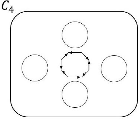
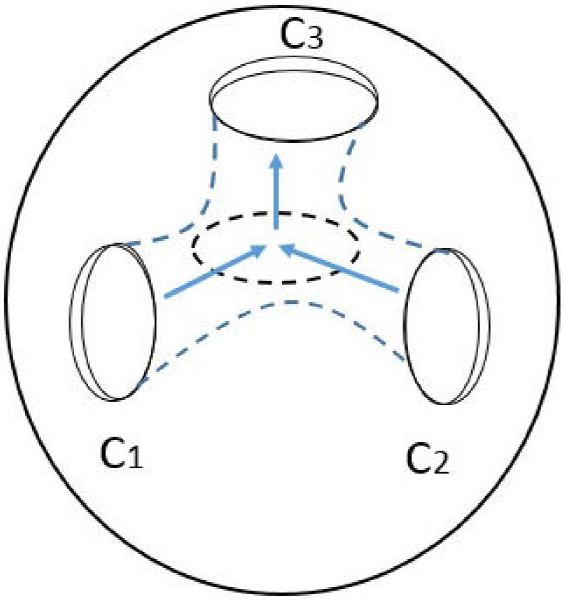
As mentioned before, topologically, the strange attractors are classified by their genus. The holes that are generated on the surface of strange attractors are determined by the fixed points of the system [¹, ², ¹⁵]. The canonical form is the topological tool that helps to know the genus of the strange attractor. This useful tool is defined as the projection of the strange attractor onto a two-dimensional (x - y plane) planar surface with g-interior holes [¹, ²]. There are two types of canonical forms that represent the surfaces of a variety of strange attractors. The first is the chain A_n (n ≥ 1) with n holes-scrolls and n - 1 separating holes with four singularities each. The genus of this canonical form is g = 2n - 1, where n s the number of holes-scroll. The second is the cycle C_n (n ≥ 2) with n holes-scrolls and one hole with 2n singularities. The genus of this canonical form is g = n + 1, where n is the number of holes-scroll [¹, ²]. Specifically, the A₂ is equal to C₂ [¹, ²], then E = A₂ = C₂. Figure 1 shows the canonical form A₁ and E, as well as Fig. 2 shows the canonical form C₄.

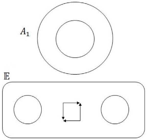
Figure 1 A ₁ depicts 1-scroll attractors with g = 1, where there is a hole without singularities. E depicts attractors with g = 3, where the attractor has 2-scrolls and one hole with four singularities. 

Figure 2 C ₄ depicts attractors with g = 5, where the attractor has 4-scrolls and one hole with eigth singularities. 

2.3. Fractional-order dynamical systems

The fundamental operator of fractional calculus is aDtα, where α and t are the bounds of the operation and α ∈ R. The operator is defined as [¹⁶]:

For α = r where r is integer, the operation 0Dtαf(t) gives the same results as classical differentiation and integration of integer-order operators. The most used approaches to define the fractional operator are the Grünwald-Letnikov (G-L), Riemann-Liouville (R-L), and Caputo. These definitions are described as follows [¹⁶]:

Grünwald-Letnikov

Riemann-Liouville

Caputo

In this work, the G-L approximation will be used for the numerical simulation of the systems.

An integer-order dynamical system can be generally defined by a set of first-ordinary differential equations of the form [¹⁷]:

where x = (x₁, x₂, . . . x_n) are the state variables and (c₁, c₂, . . . c_k) are the control parameters of the system. From a topological point of view, a dynamical system consists of a topological space Σ also called surface, a time t ∈ R and an evolution operator Φ : Σ × R → Σ [¹⁸]. In these types of Σ depends on the control parameters [¹⁷].

A fractional-order dynamical system is an extension of the definition of integer-order dynamical system. It is defined as a set of non-integer order differential equations and is described as follows [¹⁹]:

Similarly, this system consists of a surface β, a time t ∈ R and an evolution ψ: β x R → β. In these types of systems, the topology of β depends on the order of the system, as shown in [¹²].

In fractional-order dynamical systems, the concept of “system order” is not stated as in the integer-order dynamical-systems case. In integer-order dynamical systems, the order of the system is equal to the number of states or set of first-order ordinary differential equations of the system. In fractional-order dynamical systems, the order of the system is equal to the sum of the orders of the differential equations that conform the system. This means, if we have a dynamical system of order 3 which is composed of three first-ordinary differential equations, this can be modified to a system where the differential equations are fractional order derivatives, hence, the order of the system is 2 + α, where 0 < α ≤ 2 [²⁰] if the three differential equations are of fractional-order, the total order is α₁ + α₂ + α₃ . In fractional systems the derivative can adopt any arbitrary real value order. A system with constant order, i.e.α₁ ≠ α₂ ≠ ... α_i is known as a commensurate order. Whilst a system with diverse orders within, i.e. α₁ ≠ α₂ ≠ ... α_i is known as an incommensurate order system [²¹].

The algorithm to solve equation (6) uses the short memory principle and is based in the G-L definition (1), the numerical scheme has the following form [¹⁶],

where Lm is the memory length, tk = (k = 1, 2, ...), h is the time step of calculation and (−1)^j (^α_j) are binomial coefficients c_j^(α) (j = 0,1, …). For their calculation the following expression is used [¹⁶]:

The general numerical solution of the fractional differential equation is as follows:

the solution to wich can be expressed as [¹⁶]

According to the literature [¹⁰, ¹⁶], the G-L approach is equivalent to the R-L and Caputo approaches. The time domain methods to simulate fractional-order systems, require higher computational cost, but are more accurate. The G-L approach has the property of short memory which reduces the computational cost. Nevertheless, this approach has the same reliability and accuracy [¹⁰] to simulate fractional-order system as time domain methods.

3.1. The Li attractor

The Li attractor is given by [²³]:

where the parameters of the system are: a = 40, c = 11/6, d = 0.16, e = 0.65, k = 55, f = 20.

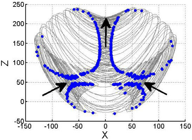
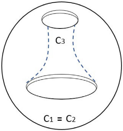
Topologically, Letellier and Gilmore in [¹⁵] define this attractor as a solid sphere pierced by two intersecting scrolls at symmetry axis, and they conclude that the genus of the attractor is 3. Therefore, its canonical form is E. The Fig. 3 shows the integer-order Li attractor of the Eq. (11) with the projection onto the x − z plane. Figure 4 shows the Poincaré section with blue color and Li’s attractor trajectories with gray color, which are spliced to show the three holes (three scrolls), the holes are pointed out by black arrows. The Fig. 5 shows an explanatory diagram where C1 and C2 are the holes that are generated in the Li attractor and the intersection of C1 and C2 generate the third hole C3.

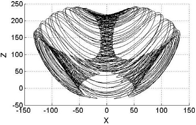
Figure 3 Simulation result onto x - z plane of the system (11) with α = 40, c = 11=6, d = 0:16, e = 0:65, k = 55, f = 20; and initial conditions (x; y₀; z₀) = (1.5; 1:5; 1.5). 

Figure 4 Poincaré section spliced with Li’s attractor trajectories 

Figure 5 Explanatory diagram of the Li attractor. 

3.2. The integer-order proto-Lorenz attractor

The proto-Lorenz attractor with 4-scrolls is given by [²²]:

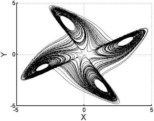
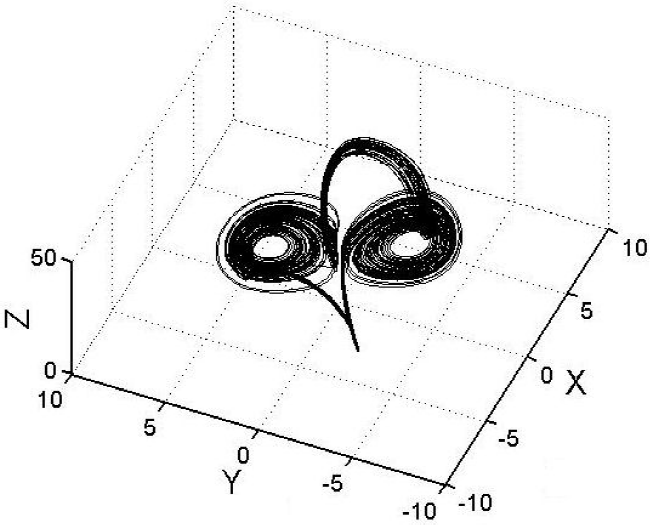
where f(x) = [−as³ + (2a + c− z)s²w + (a − 2)sw² − (c− z)w³] and f(w) = [(c− z)s³ + (a− 2)s²w + (−2a− c+ z)sw² − aw³]. The control parameters are: (a, b,c) = (10,8 / 3,28). The Fig. 6 shows the 4-scrolls strange attractor in R³ of the system (12) and the Fig. 7 shows the projection onto x − y plane of the system (12).

The Fig. 7 clearly shows that the attractor has 4 scrolls, according to [¹, ²], the canonical form that depicts this attractor is the C₄. The Fig. 2 shows this canonical form, the attractor has 4-scrolls and one hole with eight (2n) singularities. Using the expression g = n + 1, we have that g = 5.

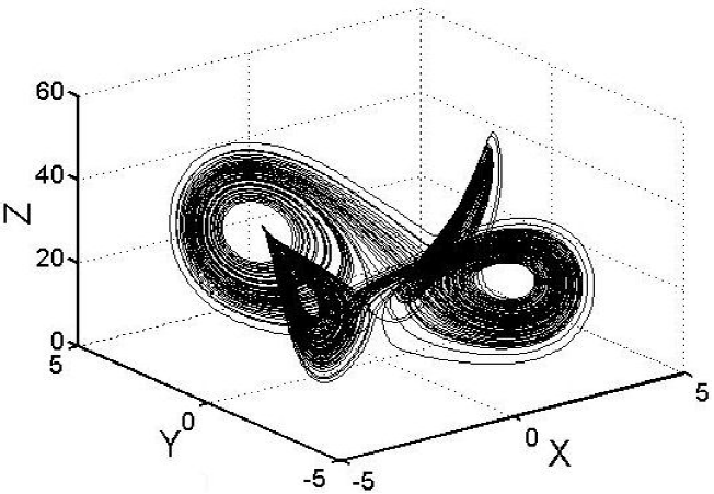
Figure 6 4-scroll strange attractor in R³ of the system (12), with (a; b; c) = (10; 8 / 3; 28) and initial conditions (s₀; w₀; z₀) = (1; 2; 6). 

Figure 7 Projection onto x - y plane for the 4-scroll strange attractor generated by system (12), with (a; b; c) = (10; 8 / 3; 28) and initial conditions (s₀; w₀; z₀) = (1; 2; 6). 

4.1. Fractional-order Li attractor

According to Eq. (6) the fractional-order Li system is defined as follows:

where the parameters and initial conditions are the same as those of the integer-order system. The order of the system α is the only parameter that changes, with incommensurate order (α₁, α₂, α₃) = (1, 0.9, 1). In Fig. 6, the new 1-scroll strange attractor generated by system 13 is shown, Fig. 9 shows the Poincaré section in blue color and trajectories of the system (13) in gray color, which are spliced in order to show the 1-hole generated within the new attractor; the hole is indicated with a black arrow. Figure 10 depicts an explanatory diagram where C1 and C2 holes come together making a single hole which connects to the C3 hole, generating a single hole or scroll.

Figure 8 Simulation result projection onto x - z plane with order (α₁; α₂; α₃) = (1; 0.9; 1). 

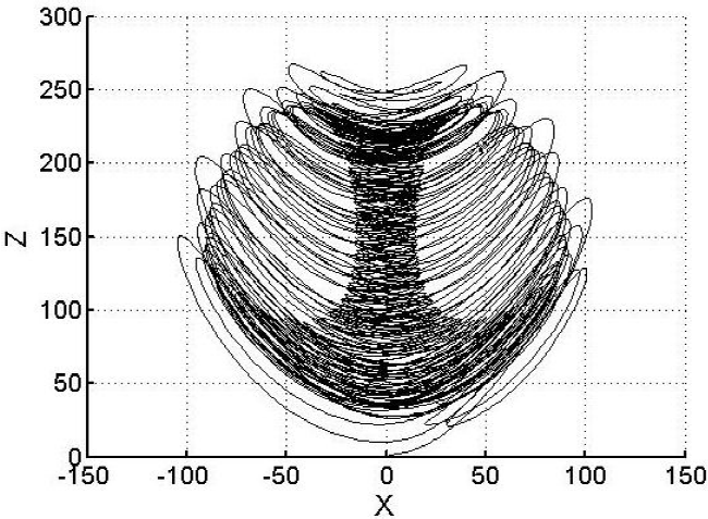
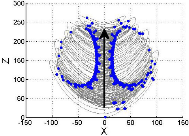
Figure 9 Poincaré section of the new 1-scroll attractor spliced with the trajectories of the system (13). 

Figure 10 Explanatory diagram of the system (13). 

It is clearly observed that the number of scrolls changes respect to system (11). This attractor has 1-scroll and belongs to the canonical form A₁, using the expression g = 2n - 1 the resulting genus is g = 1.

4.2. Fractional-order proto-Lorenz attractor

According to the Eq. (6) the fractional-order proto-Lorenz system is defined as follows:

where f(x) = [−as³ + (2a + c − z)s²w + (a − 2)sw² − (c − z)w³] and f(w)=[(c − z)s ³ + (a − 2)s²w + (−2a− c+ z)sw² − aw³]. The control parameters and the initial conditions are the same as for the system (12). With order (α₁, α₂, α₃) = (1.15, 0.7, 1.15), the system (14) generates a new 2-scroll strange attractor, as shown in Fig. 11.

Figure 11 Simulation result of system (14) in R³ with α₁ = 1.15, α₂ = 0.7, and α₃ = 1.15. 

It is clearly observed that the number of scrolls changes with respect to system (12). This attractor has 2-scroll trajectory, as mentioned before A₂ = C₂, using the expressions g = 2n − 1 and g = n + 1 the result is g = 3 therefore, its canonical form is E.

Please notice that in the results for the fractional-order Li and Proto-Lorenz attractors, the only modified value is the order of the system. Parameters and initial values remain the same.