


 text new page (beta)
 English (pdf)
 Article in xml format
 Article references
 Send this article by e-mail
 Cited by SciELO
  Similars in
SciELO
Similars in
SciELO 
 Permalink
1. Introduction
The idea of using the quantum mechanics as a calculation tool arose from the pioneering works of Feynman and Deutsch [1,2] in the 80s. It is based on the use of properties as superposition and entanglement for the realization of computational task. This requires a quantum computer that works at the microscopic level. This way, a quantum computer could solve certain known problems, more efficiently than can be done with classical computers [3], enabling advances in cryptography, drug research and development, faster data analysis, and improve artificial intelligence [4].
Major companies such as Google, Intel, Microsoft and IBM, among others, have embarked on the building of quantum computers, being able to handle up to a several tens of qubits today. In particular, the IBM Q machine used here, is a scalable quantum computer, based on superconducting technology that has the advantage of being open access through the internet [5].
Several algorithms based on quantum advantage have been proposed; among the most important are the Grover algorithm and the Shor factoring algorithm. The Grover algorithm [6] is a search algorithm of an element in a disordered base. The known classical algorithms are of order O(N), while the quantum algorithm allows to determine with high probability the desired element with an order
However, the fact that quantum systems cannot be completely isolated from the environment, together with systematic imperfections on gate applications, inexact state preparations, and inaccurate measurements, induces errors in any quantum computational task [8,9]. While there is a faulttolerant methods based on the correction of errors below a certain threshold [10], these methods are very expensive in computational resources. In other hand, the development of new tools in order to characterize and analyze the effect and propagation of quantum errors is an important issue in order to try correct them with the least possible complexity.
In this article, we analyze the error propagation in the Deutsch algorithm (DA), a special case of the general Deutsch-Jozsa algorithm [11], implemented in the quantum computer ibmqx4 (IBM Q). Some authors have implemented this algorithm in the IBM Q computer (for example to solve a learning parity problem [12,13]) but only some work has been done modeling the error of this technology [14]. The mixed state resulting from the algorithm is determined, and the error is characterized using an isotropic index [15], and is then modeled by a standard Generalized Amplitude Damping error (GAD) and a misalignment unitary error model(MA).
The public interested in research in the area of quantum algorithms, must be aware of the need to identified and model the errors, to ultimately correct and/or control them to obtain a satisfactory result.
2. Quantum computing overview
2.1 States
The qubit, the unit of quantum computation, denoted by |ψ⟩, is analog to a bit in a standard computation, and it is represented by a unitary vector, called a pure state. For example, for one qubit state, the vector |ψ⟩ = α|0⟩ + β|1⟩, is a linear superposition of vectors |0⟩ and |1⟩, where α and β are complex numbers that meet |α|2 + |β|2 = 1. The vectors |0⟩ and |1⟩ are defined in the computational base as [16]
A pure state of several qubits, is expressed as the linear combination on complex field of Kronecker product [17], of states of one qubit, denoted here by ⊗. For example for two qubits, any pure state is represented by a vector |ψ⟩ = α|0⟩ ⊗ |0⟩ + β|0⟩ ⊗ |1⟩ + γ|1⟩ ⊗ |0⟩ + δ|1⟩ ⊗ |1⟩, where α,β,γ,δ are complex numbers and the vector has unitary norm.
2.2. Evolution of states
The evolution of a quantum closed system is a reversible process, and can be represented by a unitary transformation U, on the state |ψ⟩, U|ψ⟩ = e iH∆t |ψ⟩ where H is the Hamiltonian of the physical system and ∆t the time duration of the process [16]. This representation is especially useful, since you can see the unitary transformations as quantum gates, similar to the role of classic gates in classical computation. Some transformations commonly used in quantum circuits are shown in the Table I.
TABLE I Common Unitary matrices.
| Gate name | Matrix representation |
| Hadamard gate |
|
| Pauli X gate |
|
| Pauli Y gate |
|
| Pauli Z gate |
|
| Cnot gate |
|
The entanglement of a composed state (more than one qubit), is a unique feature of quantum states, that has no analogy on classical computing. For example, the two qubit state GHZ [16] is a state of maximum entanglement which can be generated by the application of a Cnot gate I to two independent qubits |ψ⟩
as illustrated in Fig. 1.

2.3. Open systems
When we have partial information of the state, i.e., we only have information of a subsystem of the total system, the state must be represented by a positive definite hermitic matrix of unitary trace, called the density matrix of a mixed state. Any pure state can be also described by a density matrix, but the inverse is not true. For the pure state |ψ⟩ = α|0⟩ + β|1⟩, the density matrix denoted by |ψ⟩⟨ψ| is
In the rest of the article we will refer to the state of the system as the representation via the density matrix.
The decoherence can be thought of as an unwanted interaction with the environment [18]. When a quantum system is open, the interaction between the system S and the environment E can be represented as a unitary matrix of the whole system. If we only have information about the system S, it can no longer be described as a unitary vector, but can be described by a density matrix, which is the statistical average of an assembly of pure states.
The quantum evolution of a closed system can still be represented by a unitary matrix. When the state is represented by a density matrix ρ, the evolution of the state is given by ρ’ = UρU † [16].
2.4. Measurements
Unlike the reversible evolution of a closed process, quantum measurement is an irreversible process that collapses the quantum state. For example, for the one qubit state |ψ⟩, the state collapses to |0⟩ or |1⟩, with probabilities |α|2 and |β|2 respectively. In general, the measurements can be represented by operators. If we restrict ourselves to projective measurements, a physical observable M, called in this context the measurement base, can be described by the projectors P i , generated by the eigenvectors of M,
where λ i and u i are the eigenvalues and eigenvectors respectively of M. Then, the probability after projective measurement of the state ρ is [16]
and the state after measurement becomes ρ’
3. Modeling quantum errors
Every computational system is unavoidably affected by errors. In particular, the implementation of gates, the preparation of states and the measurement, can have systematic errors [19], as well as errors due to the interaction with the environment, called decoherence errors [18]. Systematic errors could be modeled as random unitary matrices, but usually they have a preferential error direction. Both type of errors can modeled by Operator Sum Representation ([20]) and characterized using the isotropic index [15].
The decoherence can be modeled by a sum of operators (Operator Sum Representation [20]) applied to the state of the system, determined to better adjust the noise for each type of technology.
A quantum operation over a state ρ denoted ε(ρ) can be expressed as a function of Kraus operators (E k ) as shown
where E
k
satisfy
3.1. Generalized amplitude damping error (GAD)
One of the standard models commonly used in the literature is a Generalized Amplitude Damping error (GAD), that could be interpreted as the interaction between a system and a thermal bath at fixed temperature. The model depends on two parameters: one related to the contact time with the thermal bath, represented as a probability of error γ ∈ [0,1], and the second related to the temperature of the thermal bath, represented by a parameter p ∈ (1/2,1]. For GAD error the Kraus operators are [16],
3.2. Systematic errors
In addition to a decoherence error, quantum computers suffer from systematic errors like classical machines. The error can be expressed by a rotation G, which could have a preferential direction in space. For example, a deviation ∈ by rotation in X direction, can be represented by the unitary matrix G = e i²X where the resulting state due to error ρ is
3.3. Isotropic error state
An isotropic error state is a mixed state that results of isotropic errors, i.e., errors that depends only of the distance from the original state, or reference state (r.s.) [15].
In the case of a n qubits reference state |0⟩ n = |0...0⟩ the mixed density matrix ρ iso representing an isotropic error state has the form
In the general case, let |ϕ⟩ be a reference state (r.s.) and M a basis change matrix so that |0⟩ = M|ϕ⟩. A mixed state ρ is an isotropic error state (r.s.|ϕ⟩) if the the state
where ρ 0 = |0⟩ n ⟨0| n and
the orthogonal isotropic mixed state relative to the reference state |0⟩ n .
Applying the inverse transform, the orthogonal isotropic mixed state of ρ ϕ = | ϕ⟩⟨ϕ | is
3.4. Isotropic index
To identify and characterize the errors, the isotropic double index defined in [15] is used. This index separates the part that cannot be corrected due to the total loss of information, called weight w, and the alignment A with respect to the expected reference state that, theoretically could be corrected.
Considering the pure reference state of n qubits, ρ
ϕ
= |ϕ⟩⟨ϕ|, and the decomposition of a state ρ after a noisy process acting on ρ
ϕ
,
• The Isotropic Alignment A,
where Fid is the fidelity between quantum states.
• The isotropic weight is
with λ being the smallest eigenvalue of ρ.
The alignment A takes values in the interval [−1,1].
When it is completely aligned with the pure reference state |ϕ⟩, A = 1, and when it is completely misaligned, A = −1. The weight take values in the interval [0,1]. When the state ρ is pure w = 0 (the inverse is true only for one qubit state) and for a state without any information, w = 1 (for one qubit state is the state maximum mixedness).
As an example, if we consider the one qubit reference state |0⟩ and the mixed state after some noisy process ρ
where
it could be realigned to the reference state
4. Error analysis on Deutsch algorithm
4.1. Deutsch algorithm
The Deutsch quantum algorithm, one of the first proposed, solves in the framework of quantum computing a problem that cannot be solved in a unique step of calculation using classical computation. Although the algorithm proposed by David Deutsch is not of immediate application, it is the basis of important algorithms based on oracles such as Grover’s search of known advantage over standard computation.
The idea is defined as follows; given a black box, known as the oracle, which consists of an unknown binary function of one bit f (x) : {0,1} → {0,1}, the goal is to decide in a deterministic way if the function is balanced or constant using the oracle only one time. The classical algorithms need two instances of application of the oracle to solve the problem in a deterministic way, while quantum Deutsch algorithm uses the oracle a single instance, as long as there are no errors in the calculation process. The Deutsch algorithm can be summarized in the following scheme shown in the Fig. 2.

Beginning with the two-qubit initial state |0⟩ ⊗ |0⟩, a X gate is applied in the second qubit getting |0⟩ ⊗ |1⟩. After applying a Hadamard transform to each qubit, the result is (1/2)(|0⟩ + |1⟩)⊗(|0⟩ − |1⟩). Applying the oracle (with one of four possible binary functions) to the current state, and ignoring the second qubit (because at this stage the qubits are independent), we get
Finally, applying a Hadamard transform to this state we have
Then it is concluded immediately that, the result is 0 for constant functions, and 1 for balanced ones.
4.2 Deutsch algorithm (DA) implementation on IBM Q
In order to analyze the performance of the algorithm in the IBM Q machine, the four possible functions of the oracle have to be implemented, i.e, f 0 constant zero, f 1 constant one, f Id identity and f NOT inverse function. Each of these functions are implemented with the previous quantum gates Table I, and are shown in Figs. 3, 4, 5, and 6.


To study the effect of the error on the resolution of the problem, the measurement of the third qubit is made (q[3]). The result in an ideal case without error, should be 0 if the function is constant and 1 if the binary function is balanced. However, the actual result is affected due to several sources of error, which distort it with respect to the ideal case. To analyze this distortion, statistical experiments were carried out, that allow us to determine in an approximate way the representative assemble of the final state, i.e., the final mixed state denoted by ρ.
4.3. Quantum state tomography (QST)
To find experimentally the density matrix of a state, a method called quantum state tomography is used [16]. Measurements must be made in the three bases (axes) of the space, X,Y and Z, to recover the density matrix state. The state ρ is given by [16]
where Tr(ρX), Tr(ρY), Tr(ρZ), are obtained, approaching the expected value by the statistical average. For example, by spectral decomposition Z = (+1)P 0 + (−1)P 1, then, Tr(ρZ) = Tr(ρP 0) − Tr(ρP 1), that by Eq. (6), Tr(ρZ) = P(0) − P(1), where P(0) and P(1) are the probabilities of measuring 0 and 1 respectively. Similar calculations were done for X and Y operators.
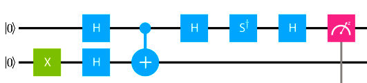
The IBM Q computer, can measure only in the canonical base (Z). Then, to measure on another base, the last two identities in Figs. 3, 4, 5, and 6, must be replaced. For example, to measure in the base X, a rotation of a q[3] qubit must be made, using in place of I d ⊗ I d , the matrix H ⊗ I d , and to measure in the Y basis, the identities must be replaced by S † ⊗ H, where
as shown in Fig. 7.
For each of the four possible binary functions, the experiments were performed 8192 times (in IBM Q computer), and the resulting density matrices and probabilities of success are obtained and shown in Table II.
TABLE II Probability of success for each binary function.
| Binary function | Resulting matrix | Ideal result | Probability |
| f 0 |
|
0 | 0.9491 |
| f I |
|
1 | 0.8503 |
| f NOT |
|
1 | 0.8252 |
| f 1 |
|
0 | 0.9495 |
4.4.Modeling GAD error in IBM Q
After a statistical analysis of experimental data, it was determined that the model that best suited this algorithm and quantum machine (IBM Q) is a Generalized Amplitude Damping (GAD) error model [15]. Running a numerical simulation of this error and comparing with experimental data, the parameters that best adjust to the Eq. (9) for the four functions at the same time are:
4.5. The misalignment error model (MA)
The resulting experimental states (IBM Q) show some misalignment with respect to the expected states (for each of the 4 functions) that cannot be modeled with a GAD error (see Table III).
TABLE III Double Isotropic Index (Weight and Misalignment as defined in Eqs. (15) and (16)) and Fidelity between the IBM Q experimental result and the simulated error model.
| Binary function | Ideal result | Weight (w) | Misalignment (A) | Fidelity |
| f 0 | 0 | 0.0873 | 0.9070 | 0.9999 |
| f Id | 1 | 0.2965 | 0.9544 | 0.9976 |
| f NOT | 1 | 0.3051 | 0.8049 | 0.9996 |
| f 1 | 0 | 0.0862 | 0.9056 | 0.9999 |
The GAD error model can generate a certain weight (w) in the pure states resulting from the algorithm, but it cannot generate a misalignment with respect to these. We propose a method that consists of a unitary transformation (rotation) applied to three qubits (two qubits of the algorithm and one auxiliary one) that quantifies the misalignment of the state.
In order to determine the appropiate rotation that has to be applied to each function, knowing the theoretical result (0 for f 0, f 1 and 1 for f I , f Not ) we generate a rotation from that state to the experimental one (G f0 , G f1 for 0 , and G fI , G fNot for 1), in the same manner as 18. Finally, an approximation to the geometric mean is applied to both cases given by
resulting in
Since the result of the algorithm is a priori unknown, the proposed model applies a conditional operator depending on the result as shown in Fig. 8.

The result of the model, quantified using the fidelity between the IBM Q experimental result and the simulated one, is shown in the Table III.
5. Results and conclusions
In this work we have modeled the propagation of errors in a real quantum machine, such as IBM Q (ibmqx4). The resulting mixed states of a quantum Deutsch algorithm, are found by means of a QST method. Through the characterization using an isotropic index, the error has been modeled, in which the loss of information is given by a GAD error model, and the misaligned part by means of unitary conditional matrix (MA error model). As shown in Table III, the largest source of error in this case is the decoherence, given by the weight (w) and modeled by GAD error model. Furthermore, the Misalignment error improves the error model bringing fidelities close to one.
The proposed error model fits very well with the experimental results, and can be the first step for the future correction of systematic errors in quantum systems.

