


 text new page (beta)
 English (pdf)
 Article in xml format
 Article references
 Send this article by e-mail
 Cited by SciELO
  Similars in
SciELO
Similars in
SciELO 
 Permalink
1. Introduction
The flow of a fluid over rotating disk has many applications in engineering and industry. Rotating bodies, centrifugal pumps, viscometers, rotors, fans, turbines, spinning disks are examples of rotating disk flows. The problems of the rotating disk are formulated in terms of nonlinear PDE’s and ODE’s. Exact solutions of these non-linear boundary value ODE’s and PDE’s are rare. Therefore, researchers are thinking about other methods for accurate solutions to nonlinear problems. Thus, the numerical methods are powerful tools for the approximate solution of such problems.
The history of rotating disk flow is very long, and von Kármán [1] was the first one who studied flow over rotating disk by mean of self-similar transformations. Later on, the momentum integral transform method is used for the solution of proposed model equations. Interesting features of analysis are highlighted that the Navier Stokes equations are transformed into a system of boundary values ODE’s and then solved by momentum integral transform method. The researchers discussed these remarkable results and retrieved the important and interesting flow patterns as a special case. Later on, Cochran [2] extended the results of [1] and obtained a better accurate numerical solution to the von Kármán problem. Stuart [3] first discussed the effects of uniform suction (blowing) on fluid motion maintained over a porous rotating disk. He obtained different results for the steady flow by considering strong suction and do not provide reasonable solutions for injection cases. Gregg and Sparrow [4] solved the mass and heat diffusion equations for viscous flow over a rotating disk. In the modeled problem, they investigated the consequences of injection on the flow properties and obtained simple asymptotic solutions for large values of the suction parameter. Benton [5] improved Cochran’s solutions and solved unsteady Navier Stokes equations for rotating flows. Kuiken [6] analyzed the cases of strong injection and presented the boundary layer solution for this case. He found the inner and outer solutions to the problem. Ackroyd [7] found an asymptotic type exponential series solution with negative exponents and showed that such solutions exhibit high accuracy for all cases of suction and low values of blowing. He also determined the radius of convergence for the asymptotic series solution. Meanwhile, Crane [8] found a closed form solution for the flow on the stretchable sheet, and Wang [9] extends it to 3−D (closed form) models. Recently, Fang [10] studied the effect of stretching on the flow over an annular rotating disk and solved the modeled equations numerically. Note that the fluid flow due to annular rotating disk are discussed in [11]. Further investigations of such flows have been considered and analyzed over here.
In this paper, we have studied the combined effects of stretching (shrinking) and injection (suction) velocities on the viscous fluid flow over a porous rotating and porous disk. Remember that the stretching (shrinking) and injection (suction) velocities are variables and depending upon the radial coordinate. The rotating velocity of the porous disk is not uniform and taken as a function of r. The governing PDE’s are converted into boundary value ODE’s by employing new and unusual similarity transformations of von Kármán type, and exact self similar equations are formed. The results of this system of ODE’s are exactly matched with the classical similarity solutions for particular cases of parameters value. These observations are recorded in different figures, which are presented in the results and discussion section. The new boundary value ODE’s, together with the boundary condition, are solved numerically. The modeled equations are exactly matched with the classical model of von Kármán for special choice of parameters value used in similarity transformation. It is also confirmed that the boundary layer is displaced for each set of parameters value; i.e. the boundary layer is remained the same, whereas the flow properties are changed with changes in size of the domain (the similarity variable η). These observations are noted in a figure given in a forthcoming section.
2. Formulation of the problem
In the current formulation, we have considered a cylindrical polar coordinate system (r,θ,z) for the flow problem such that the velocity vector has three components (u r ,u θ ,u z ). Further, it is assumed that the flow is axi symmetric i.e. the unknown quantities are independent of θ. Note that u r ,u θ , and u z are velocity components in r,θ and z directions, respectively. The geometry of the problem is so chosen that infinite porous annular disk is lying in the plane z = 0, rotates about the z-axis, and enters/ exits fluid in the z-direction. The disk is also stretched (shrunk) in the r direction with proper and the variable stretching (shrinking) velocity U r (r). The disk is also rotating with variable angular velocity Ω(r). Recall that the non-uniform porous disk allows variable injection (suction) velocity U z (r). The governing equations of motion consist of the continuity equation and three components of momentum equations. For in compressible and axi symmetric flow in cylindrical polar coordinates, the continuity equation has the following form:
r momentum equation is:
θ momentum equation is:
z momentum equation is:
the no-slip and ambient boundary conditions are obtained from the physical geometry of the problem:
at
where ρ, ν, and p are fluid density, kinematic viscosity, and pressure, respectively. The different known quantities are defined such that: U r (r) = U 0 /r, U z (r) = V 0 /r, Ω(r) = W 0 /r 2 where U 0 > 0(< 0), V 0 > 0(< 0), W 0 are stretching (shrinking), injection (suction), and rotation parameters, respectively. Remember that, U 0, V 0, and W 0 have the dimension of L 2 /T. Here, we assumed the new and unusual similarity transformations for the velocity components and pressure. The new variables are formed because of the boundary conditions of the modeled problem. Therefore, they encompasses all the features of the problem. Note that the variable angular velocity is characterized by the radius of the disk. All these information are incorporated in the similarity transformations and finally we get the following form:
The new variables in Eqs. (6) are further simplified by choosing numerical values for the parameters c 0 = 0, c 2 = −1, A = ν and finally we get:
By substituting the variables from Eq. (7) into Eqs. (1 − 4), we obtained the following system of ODE’s:
where prime denotes the derivative concerning η. By substituting the definitions from Eq. (7) into Eq. (5), we have:
where U 0 /ν = α 1 > 0 (< 0) V 0 /ν = α 2 > 0 (< 0) and α 3 = w 0 /ν are stretching (shrinking), injection (suction), and rotation parameters, respectively. A subsidiary condition is obtained from Eq. (8) by integrating it between δ and ∞ and gives:
3. Comparision with von Kármán’s problem
The classical von Kármán problem can be easily recovered by adjusting the parameters of new variables defined in Eqs. (6). Moreover, we assumed the following particular value for the parameters:
Because of the above value for the parameters, the transformations in Eq. (6) are exactly converted into the von Kármán’s variables defined for velocity components and´ pressure:
Where
The boundary conditions in Eq. (5) are recovered for von Kármán problem given Eqs. (13- 14) and we get:
Numerical solution of Eqs. (15-19) is obtained by the bvp4c package in Matlab and presented in Fig. (1) and Table I. The unknown quantities F,G,H and −P are plotted against the similarity variable η and exactly matched with a published solution of von Kármán problem given in F. M. White [12]. Similarly, the numerical data for the von Kármán problem is presented in Table I. In this table, the numerical values of F,F’,G,G’,H,−P are calculated at different values of η and the data is exactly matched with published results of von Kármán problem.
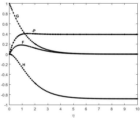
FIGURE 1 Comparison of the numerical solution (dotted lines) of Eqs. (14-18) with the von Kármán solutions (solid lines).
TABLE I Numerical solution of von Kármán problem in Eqs. (13-17).
| η | F(η) | F’(η) | G(η) | G’(η) | H(η) | -P(η) |
| 0.051 | 0.0246 | 0.4586 | 0.9686 | -0.6137 | -0.0013 | -0.0493 |
| 0.4082 | 0.1371 | 0.1929 | 0.7579 | -0.555 | -0.0647 | -0.2762 |
| 0.8163 | 0.1774 | 0.0245 | 0.5537 | -0.4432 | -0.1977 | -0.3744 |
| 1.0204 | 0.1773 | -0.0222 | 0.4691 | -0.3863 | -0.2704 | -0.3912 |
| 1.1905 | 0.1712 | -0.0478 | 0.4072 | -0.3418 | -0.3298 | -0.3969 |
| 1.5986 | 0.1448 | -0.0756 | 0.2872 | -0.2497 | -0.4596 | -0.3951 |
| 2.0068 | 0.1131 | -0.0766 | 0.2003 | -0.1797 | -0.5648 | -0.3857 |
| 2.2109 | 0.0979 | -0.0722 | 0.1665 | -0.152 | -0.6079 | -0.3805 |
| 2.415 | 0.0837 | -0.0664 | 0.138 | -0.1285 | -0.6449 | -0.3754 |
| 2.7891 | 0.0611 | -0.0543 | 0.0966 | -0.0944 | -0.6988 | -0.3664 |
| 2.9932 | 0.0507 | -0.0479 | 0.0789 | -0.0798 | -0.7216 | -0.3617 |
| 3.1973 | 0.0416 | -0.0418 | 0.0639 | -0.0675 | -0.7403 | -0.3572 |
| 3.6054 | 0.0267 | -0.0312 | 0.0405 | -0.0484 | -0.7679 | -0.3483 |
| 4.0136 | 0.0158 | -0.0229 | 0.0237 | -0.0348 | -0.785 | -0.3396 |
| 4.2177 | 0.0114 | -0.0196 | 0.0171 | -0.0295 | -0.7906 | -0.3353 |
| 4.5918 | 0.0051 | -0.0146 | 0.0076 | -0.0218 | -0.7966 | -0.3275 |
| 4.7959 | 0.0023 | -0.0124 | 0.0035 | -0.0186 | -0.7981 | -0.3232 |
| 5 | 0 | -0.0105 | 0 | -0.0158 | -0.7986 | -0.3189 |
4. Results and discussion
The numerical solution of Eqs. (8-12) is presented here and obtained by the R-K method coupled with a non-linear Shooting Method [13]. The scheme is developed by Cebeci and Keller [14] and widely used for the solution of such problems. The effects of all parameters are seen on the representatives of velocity components and pressure distribution.
All the figures are obtained from the solution of Eqs. (812) and the infinity boundary conditions are satisfied asymptotically. These facts are providing the validity and correctness of the numerical solution. Here, we discussed the numerical solutions of the final equations, and the consequences of different parameters are seen on field and flow quantities. However, we elaborated the basics and fundamentals of the three dimensional von Kármán type flow over a porous, rotating disk, which were combined with the effects of stretching (shrinking) and injection (suction) velocities. In Figs. 2-6, the velocity components F,G,H and G’ (gradients of tangential velocity) are presented for different fixed values of α 1 , α 2 , α 3. It is observed that F and H are decreased with the increasing of α 1. The profiles in these graphs are approached to zero as the similarity variable (η) is reaching infinity. The unknown functions F and H are negative at some points in the domain of similarity variables η that correspond to reverse flow, and these functions necessarily obtained minimum values. Each profile in Fig. 2 (a) has a nadir, and the minimum values of the function F are such that F(0.8163) = −0.2753, F(0.8163) = −0.4878, F(0.7755) = −0.6893, F(0.7755) = 0.8810, F(0.8163) = −1.0640, respectively. Note that the minima for F are varied in the range [−1.0640 − 0.2753]. The largest negative velocity is noted for α 1 = 3 at η = 0.8163 which is −1.0640.
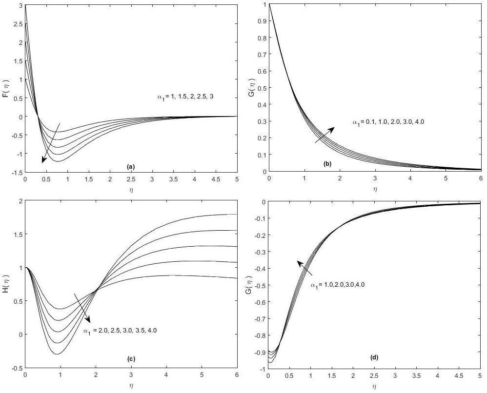
FIGURE 2 Effects of stretching parameter α 1 > 0 on (a)F,(b)G,(c)H,(d)G’ are seen for α 2 = 1;α 3 = 1.0
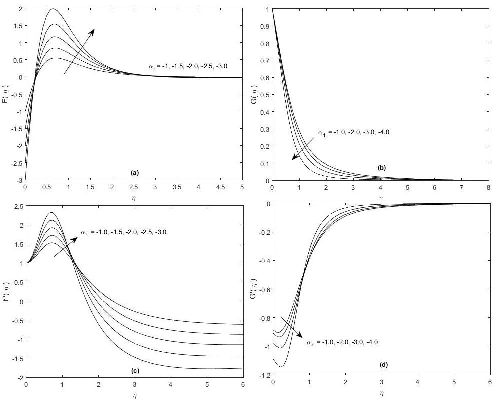
FIGURE 3 Effects of shrinking parameter α 1 < 0 on (a) F, (b) G, (c) H, (d) G’ are seen for α 2 = 1,α 3 = 0.3
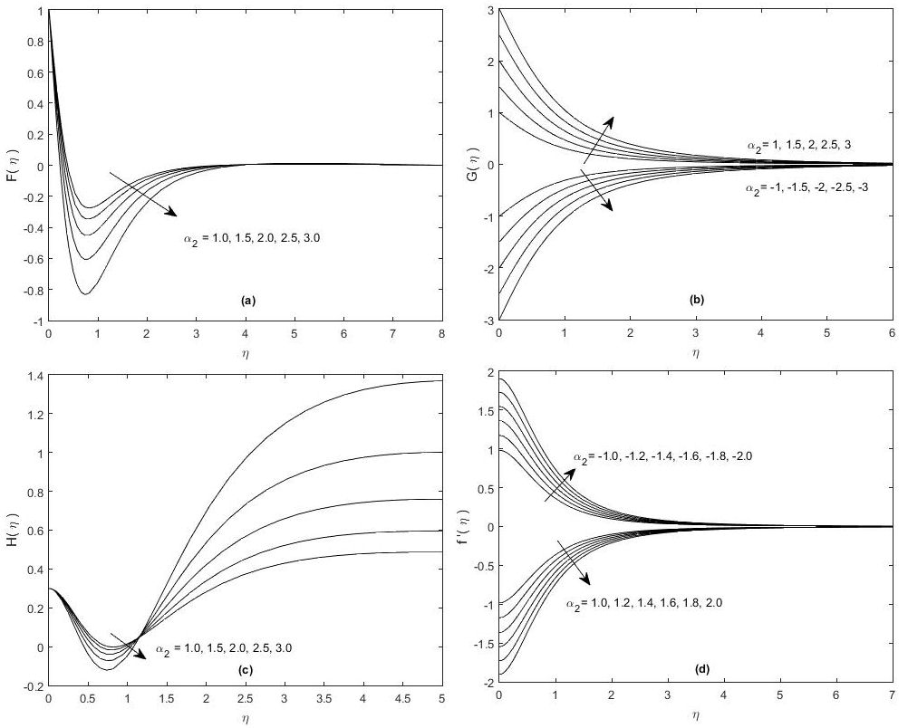
FIGURE 4 Effects of rotation parameter α 2 > 0 on (a) F, (b) G, (c) H, (d) G’ are seen for α 1 = 1,α 3 = 0.3.
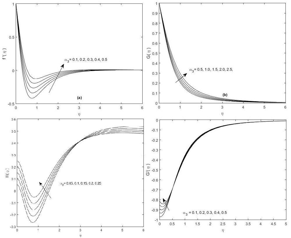
FIGURE 5 Effects of injection parameter α 3 > 0 on (a) F, (b) G, (c) H, (d) G’ are seen for α 1 = 1,α 2 = 1.
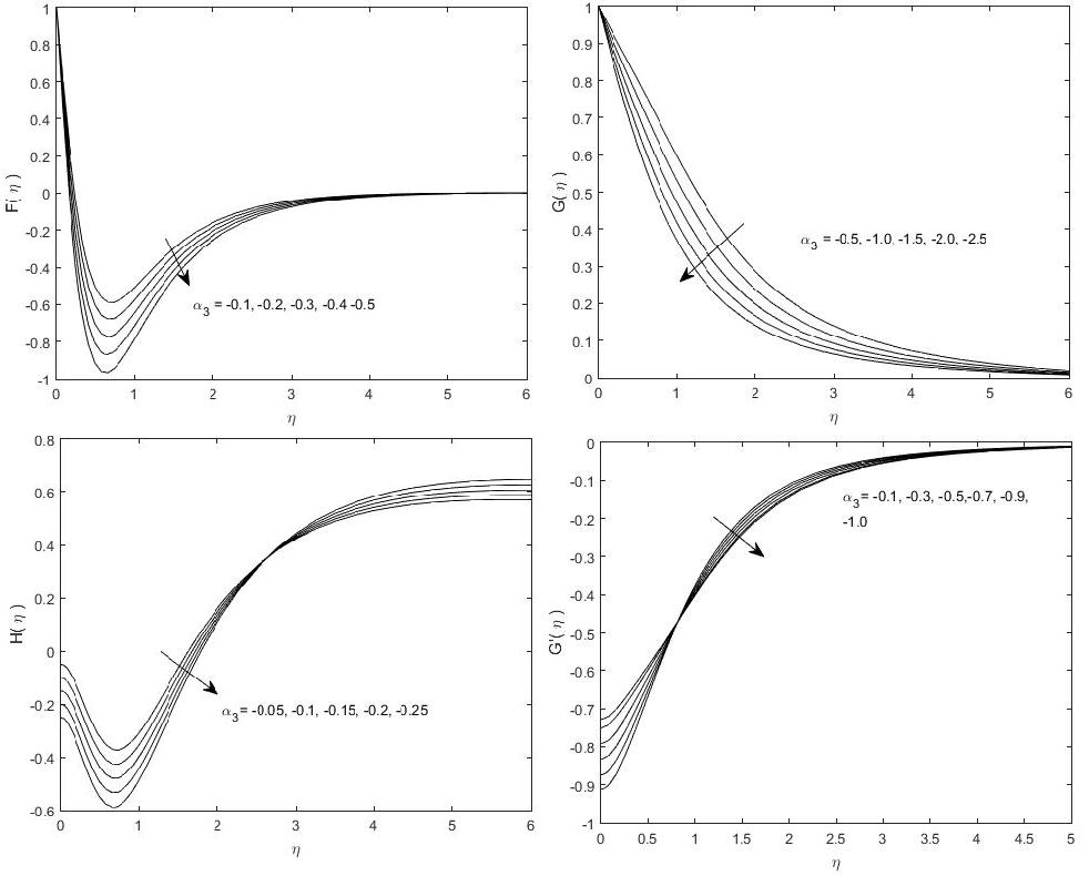
FIGURE 6 Effects of suction parameter α 3 < 0 on (a) F, (b) G, (c) H, (d) G’ are seen for α 1 = 1,α 2 = 1.0.
In Fig. 2 (b), the velocity component G is not changed with α 1, near the surface of the disk, and minor changes have been seen in its profiles away from the disk’s surface. The profiles of G are purely asymptotic in nature. It is also confirmed from the figure that F is attained its maximum value for small values of the similarity variable η. Figures 2 (a) and 2(c) represent that F(η) and H(η) have obtained their minimum values immediately near the surface of the disk. The profiles in these two figures are increased monotonically with the increasing of the boundary layer thickness. However, this behavior is opposite for the shrinking disk, and the facts are shown in Figs. 3(a) and 3(d). The tangential velocity G(η) and its derivative (G’(η)) are decreased (increased) with the increasing of α 1, as shown in Figs. 3(b) and 3(d), but these changes are very small as compared to the changes in F and H due to the variation of α 1.
In Figs. 4(b) and 4(d) effects of α 2 > 0, and α 2 < 0 are observed on G and G’, respectively. In both the figures G (G’) is increased with increasing (decreasing) of α 2 > 0 (α 2 < 0) and decreased with the decreasing (increasing) of α 2 < 0 and α 2 > 0. There are two groups of profiles in these two figures. In Fig. 4 (b) and 4(d), the positive profiles are corresponding to α 2 > 0 (α 2 < 0) while the negative profiles are associated with α 2 < 0, α 2 > 0. The decay of G and G’ is noted in the first branch in Figs. 4(b) and 4(d) for α 2 > 0 and α 2 < 0, respectively. It is seen that the profiles in one group are the reflection of others about the similarity line, and each group is corresponding to the positive and negative values of α 2 > 0. In Figs. 5(a), 6(a), F is increased with the increase of α 3 > 0 and decreased with the decrease of α 3 < 0. Both F and H are attained their minimum values near the surface of the disk. It is also noted that H is converged to a constant number asymptotically, depending on the value of α 3. The tangential velocity component G and its derivative G’ are increased with the increasing of α 3 > 0. In Fig. 6(b), it is observed that the suction velocity gives rise to the famous inflection point profiles for G’. In the presence of suction, the axial velocity outside the boundary layer is greater than for non-porous disk. Note that the large injection velocity is opposing the inflow at the same rate. The centrifugal weights due to the rotating disk have also appeared which causes suction. It is also confirmed that the fluid in the vicinity of the disk is rotating faster than the disk. The decay of circumferential velocity is noted in each case, and necessarily, it is the obvious contribution of viscous diffusion.
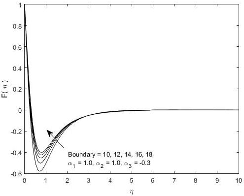
In Fig. 7 (a-d) effects of α 1 > 0,α 1 < 0, α 2 > 0, and α 3 > 0 are shown on P, respectively. In Fig. 7 (b), the profiles of pressure distribution are risen to the maximum value at η = 0.3265 and then decreased slowly and gradually to zero for α 1 = −3, −2.5, −2, −1.5, −1. In this figure, the highest peak of the profile is observed for large negative values of α 1(the shrinking parameter). On the other hand, the pressure distribution is dropped in Fig. 7 (a) for α 1 < 0 and in Fig. 7 (c) for α 2 > 0. The profiles have nadir for large values of α 1 < 0 and α 2 > 0 at η = 0.3265. In both the figures, the pressure drop is increased with the increasing of these parameters. Similarly, in Fig. 7 (d) pressure is plotted against η for different values α 3 > 0. The pressure drop is uniformly decreased with the increasing of α 3. The variation in the pressure drop due to α 3 is significantly small as it is compared to the changes in other parameters. In Fig. 8, the boundary layer displacement is noted. For fixed values of all parameters, abrupt changes are recorded in the velocity profiles, with the changes in boundary size. In this figure, each profile is approached zero asymptotically. The velocity is increased with the increasing of boundary size, whereas the boundary thickness is not changed. All the patterns in the profiles are similar. It just shifts to the new position. The depth of penetration of the axial velocity is increased with increasing of α 1 > 0,α 2 > 0,α 3 < 0 and decreased with the increasing of α 3 > 0.
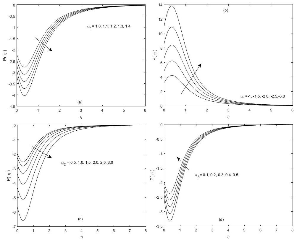
FIGURE 7 Effects of stretching (shrinking), rotation and injection (suction) parameters are shown on P.
4.1. The thickness of the boundary layer
The thickness of the boundary layer is evaluated numerically from Figs. 2, by considering the standard definition, widely used in the literature. In Figs. 2, 4, and 6, the thickness of the boundary layer decreased with the increasing of α 1 > 0,α 2 > 0 and α 3 < 0, respectively. Similarly, in Figs. 3 and 5 the thickness of the boundary layer is increased with the increasing of α 1 < 0 and α 3 > 0, respectively. Moreover, the boundary layer’s thickness is strictly varied with the changes in parameter values.
The details of the boundary layer thickness are provided in Table II, below. It is confirmed that the thickness of boundary layer may be evaluated by considering the tangential velocity component or G(η). Note that the current observations ar/e not similar and analogous to the classical von Kármán problem. The thickness of the boundary layer δ 0 is behaved differently, contrary to the classical observations.
TABLE II The thickness of boundary layer is determined from Figs. 2-6.
| α 1 ↓,α 2 = 1.0,α 3 = 0.3 |
|
α 3 ↓,α 1 = 1.0,α 2 = 1.0 |
|
| 1.0 | 5.5782 | 0.1 | 5.4422 |
| 1.5 | 5.4442 | 0.2 | 5.5102 |
| 2.0 | 5.2891 | 0.3 | 5.5782 |
| 2.5 | 5.068 | 0.4 | 5.6463 |
| 3.0 | 4.932 | 0.5 | 5.6973 |
| -1.0 | 6.4626 | -0.1 | 5.2041 |
| -1.5 | 6.6667 | -0.2 | 5.1361 |
| -2.0 | 6.9728 | -0.3 | 5.0680 |
| -2.5 | 7.1769 | -0.4 | 5.000 |
| -3.0 | 7.4830 | -0.5 | 4.9320 |
| α 2 ↓,α 1 = 1.0,α 3 = 0.3 |
|
||
| 1.0 | 5.5782 | ||
| 1.5 | 5.5782 | ||
| 2.0 | 5.4592 | ||
| 2.5 | 5.4592 | ||
| 3.0 | 5.3571 | ||
5. Conclusion
Other interesting features of the flow are explored and summarized by calculating the torque (experienced by a disk) when the disk has large but finite radius R :
The individual and combined effects of four different parameters have seen on rotating disk flows. The physical interpretation of all these parameters depends upon their signs (either these are negative/ positive or zero, and their consequent effects are seen on field quantities). The new observation is summarized in different figures of the discussion section, more precisely, the classical observation of von Kármán is the special case of this study. The current formulation also unifies a set of models which correspond to suction/injection, through rotating disk with stretching/ shrinking effects. Note that the boundary layer is displaced to right (left) against the parameters α 1 > 0,α 2 > 0,α 3 > 0 (α 1 < 0,α 2 < 0,α 3 < 0) and a special result has been plotted in Fig. 8 and other cases are not included here.

