SciELO - Scientific Electronic Library Online

 
vol.66 issue2Quantitative and qualitative analysis of segmental dielectric relaxations and space charge by TSDC in nanocomposites of natural rubber/clayNonlinear mixed convective nanofluid flow along moving vertical rough plate author indexsubject indexsearch form
Home Pagealphabetic serial listing  

Services on Demand

Journal

Article

Indicators

Related links

  • Have no similar articlesSimilars in SciELO

Share


Revista mexicana de física

Print version ISSN 0035-001X

Rev. mex. fis. vol.66 n.2 México Mar./Apr. 2020  Epub Mar 26, 2021

https://doi.org/10.31349/revmexfis.66.137 

Research

Fluid Dynamics

Transient analysis of combined electroosmotic and pressure-driven flow with multi-layer immiscible fluids in a narrow capillary

D. Torresa 

J. Escandóna  * 

aInstituto Politécnico Nacional, SEPI-ESIME Azcapotzalco, Departamento de Termofluidos, Av. de las Granjas No. 682, Col. Santa Catarina, Alcaldía Azcapotzalco, Ciudad de México, 02250, México.


Abstract

Because there is required the development of techniques for pumping parallel flows in miniaturized systems, in the present investigation is obtained a semi-analytical solution based in the matrix inverse method and by Laplace transform, for the transient flow of multi-layer immiscible fluids in a narrow capillary under electroosmotic and pressure driven effects. The dimensionless mathematical model to solve the electric potential distribution and the velocity field in the start-up of flow, consists of the Poisson-Boltzmann and momentum equations, respectively. Here, the transported fluids are considered symmetrical electrolytes. Also because the interfaces between them are polarizable and impermeable to charged particles, interesting interfacial effects appear on the velocity profiles when an external electric field is applied. The results show graphically the influence of the different dimensionless parameters involved in the dynamics of the fluid flow. This study demonstrates that by considering interfacial electrical effects at the contact between two electrolytes, a steep velocity gradient is produced resulting in strong changes in the velocity whose magnitude and direction depending on the concentration and polarity of electric charges around a liquid-liquid interface; finally, it is observed that the time to reach the steady-state regime of the fluid flow is only controlled by the dimensionless viscosity ratios. This investigation is a theoretical contribution to simulate transient multi-layer fluid flows under electric interfacial effects, covering different implications that emerge in the design of small devices into the chemical, biological, and clinical areas.

Keywords: Transient electroosmotic flow; immiscible fluids; narrow capillary; interfacial effects; multi-layer flow

PACS: 47.10.-g; 47.57.jd; 68.05.-n; 68.08.-p; 82.45.Gj

1. Introduction

The concept of integrating biochemical analysis with microelectromechanical systems (MEMS) is involved in the new field of bioMEMS, which is undergoing tremendous growth in a multitude of applications [1], including technology that enable scientific discovery, detection, diagnostics, and therapy and span the fields of biology, chemistry, and medicine [2]. In this context, the terms lab on a chip (LOC) and micro total analysis system (µTAS) are a subset of MEMS dedicated to chemical and biological analyses and discoveries [2]; here, the study of fluid flow in these submillimeter-sized systems is cover by microfluidics and nanofluidics [3].

In the mentioned systems can be applied different strategies to pump fluids as electrohydrodynamic and magnetohydrodynamic effects [4,5], electrothermal effects [6], acoustic and ultrasonic effects [6, 7], pressure-driven effects by syringe, peristaltic or rotary pumps [8], among others [6]. However, a common method for pumping fluids is the use of the electrokinetic phenomenon called electroosmosis, whose basic principle is the movement of an electrolytic solution relative to a stationary charged surface when an electric field is applied [9].

Focusing on electroosmotic flows, these have been studied extensively by the scientific community since many years, carrying investigations about the transport of homogeneous single-phase fluids based in electrolytic solutions both steady-state and transient-state, and using conduits formed with cylindrical shape [10-12], annular channels [13-15], parallel flat plates [16-18] and rectangular channels [19-21]; all of them, under the consideration of the Debye-Hückel approximation for the volumetric free charge density within the electric double layer.

The research about electroosmotic flows, have been extended to the study of the pumping of two parallel and immiscible fluids as a technique of transport by viscous drag. In this direction, Liu et al. [22] refer that non-conducting liquids and certain biofluids cannot be pumped directly by electroosmosis, but still can be dragged along by shear forces of a neighboring conducting liquid which is driven by electroosmosis. Their study reports an analytical solution for the velocity profiles into a two-phase electroosmotic-viscous pump in a circular microchannel. About this theme, other investigations under electroosmotic effects to pumping a nonconducting fluid by viscous drag due to electroosmotic effects over a conducting liquid in cylindrical channels can be reviewed in the works conducted by Movahed et al. [23], Moghadam [24] and Matías et al. [25]; moreover, in parallel flat plates by Huang et al. [26] and Afonso et al. [27], and rectangular channels by Gao et al. [28]; all of them in steadystate. Concerning the transient-state analysis of pumping of non-conducting liquids by viscous drag induced by electroosmotic effects, we can cite the investigation realized by Gao et al. [29] in a rectangular channel.

All the studies cited in the above paragraph consider that one of the fluids in the two-layer arrangement is electrically conducting and the other not, which yields partially or null employment of the Maxwell electric stresses at the liquidliquid interfaces between fluid layers. However, following the study of the electrochemistry, if two solutions of immiscible electrolytes are in contact and develop a polarizable and impermeable interface to charged particles, there arises, in equilibrium, an electrical potential difference, whose structure trough diffuse layers and a compact inner layer in an electrical double layer, has been studied by Volkov et al. [30], Wandlowsky et al. [31], Samec et al. [32] and Cui et al. [33]. In the mentioned works, the electrical potential difference is determined by the distribution of charged and dipolar particles near the interface. However, Masliyha and Bhattacharjee [9], propose a simpler contact structure between the immiscible media, where the thin compact layers or the presence of electrical dipoles are not considered; therefore, the potential difference can be considered as a constant and when this constant is zero the electrical potential continuity is reached.

Another important aspect that emerges in the analysis of the structure of the electric double layer in polarizable, and non-polarizable interfaces, is the study of capacitance, which is a measure of the penetration of ions in the electric double layer at the interface. From the capacitance and the potential difference, the surface charge density at the interface can be determined [32, 33]; therefore, the potential difference and surface charge density have a direct correspondence when two immiscible electrolyte solutions are in contact through an interface.

Considering the previous paragraph about certain concepts involved within the double electric layer generated at the interface between two immiscible electrolyte solutions, the studies of Choi et al. [34], Su et al. [35] and Jian et al. [36] carry out the analysis of the transient electroosmotic flow of two-immiscible fluid layers in slit channels formed by parallel flat plates. Here, both fluids are electrolytes, and this condition leads to the Maxwell electric and shear stresses be included in each fluid phase when the total stresses balance is established at the liquid-liquid interface. The flow field experiments important changes in their velocity profiles when the electric stresses are present at the interface concerning to the case when only one fluid is conductive, due to the presence of a potential difference and a surface charge density in the interfacial boundary conditions. Extending the mentioned works, Shit et al. [37] realized a study in steady-state about the two-layer fluid flow and heat transfer in a hydrophobic microchannel formed by parallel flat plates using a combination of a pressure gradient and electroosmotic forces. Their results indicate that the effects of the interfacial zeta potential are significant on the fluid velocity; moreover, the electroosmotic flow has a finite jump the interface between two fluid layers.

Certainly, the development of techniques to pumping immiscible fluids by electroosmotic effects in miniaturized systems has reached the handling of three layers of fluids [38] and also any number of fluid layers [39], when the flowfocusing effect is required. Therefore, the aim of the present work is addressing the study about the transport of multilayer immiscible fluids in a cylindrical capillary under pressure and electroosmotic effects. The parametric study on the flow field is focused on the interfacial phenomena via a potential difference, the Gauss’s law, and Maxwell stress at each liquid-liquid interface between fluid layers. Because the interface conditions established here for the star-up of a multilayer flow within a capillary have not been treated yet, this paper also has the purpose of extending the theoretical knowledge about the application of the electrokinetic phenomena in fluids transport.

2. Mathematical formulation

2.1. Physical model

In the present work, we realize the transient analysis of the transport of multi-layer immiscible fluids in a narrow capillary. Therefore, to establish the fluid phenomenon that will be studied here, we start describing the physical model with a cylindrical coordinate system (r,z), as is shown in Fig. 1 on the centerline of a capillary. The fluids, which fill the conduit with radius R, are layers of symmetrical electrolytes consider with a Newtonian behavior. Each liquid-liquid interface is placed in an r n position; here, the subscript n = 1,2,3,...,i represents the number of the fluid layer, and i is the fluid layer in contact with the wall of the capillary. Because the fluids are immiscible and electrically conductive, and also the interfaces between them are polarizable and impermeable to charged particles, a surface electric charge density q s and a potential difference ∆ψ appears at the liquid-liquid interfaces; moreover, the wall of the capillary is also polarizable and acquire a surface electric charge represented by the zeta potential ζ w . The fluids movement is due to two factors; firstly, to the ends of the conduit, and is subject to an electric potential generated by a pair of electrodes, that gives rise to a uniform electric field E z inducing electroosmotic effects. Secondly, by a pressure gradient p z , that also could be applied along the z−direction.

FIGURE 1 Sketch of the combined electroosmotic and pressuredriven flow of multi-layer fluids in a capillary. 

2.2 General governing equations

The flow field of the multi-layer immiscible fluids is governed by the Poisson-Boltzmann equation for the electric potential distribution

2Φn=-ρenϵn, (1)

where Φ is the total electric potential, ρ e is the volumetric free charge density and (( is the dielectric permittivity. Also, with the continuity equation for incompressible fluids as

vn=0, (2)

being v the velocity vector. And the momentum governing equation

ρnDvnDt=-p+μn2vn+ρng+ρenE, (3)

where ρ is the density, t is the time, p is the pressure, µ is the viscosity, g is the gravitational acceleration, and E is the electric field vector.

2.3 Simplified mathematical model

The mathematical model to solve this multi-layer flow based on the previous general governing equations can be simplified, taking into account the following assumptions:

  • Incompressible fluids.

  • The fluid’s properties are independent of the local electric field, ion concentration, and temperature [22,40]. Complementary to this consideration, we assume a net change in the temperature of the fluids is less to 10 K [41, 42] and the value of the external electric field is less to 10 kVm−1 to despise any Joule heating effect [43].

  • The interfaces between the fluids represent either sharp boundaries with zero-thickness, impermeable, and ideally polarizable.

  • There is a planar interface between fluids layers [34, 44]. The mentioned can be assumed by considering that we have: i) laminar flow for low Reynold’s numbers, being Ren(=ρnRvc/μn)1, resulting in parallel flows with laminar fluid interfaces [38] and ii) uniform zeta potential along the wall of the capillary. Here, the characteristic velocity of the flow is defined by vc=-ϵrefζwEz/μref, where the subscript “ref” indicates physical properties referred to electrolytes in aqueous solutions at 298.15 K (25 C) [9,45].

  • The gravitational forces in the system are negligible [44].

  • The capillary is sufficiently long, and the analysis is a focus in a region far from the ends of the capillary neglecting inlet and outlet effects.

  • For a long capillary, the total electric potential Φ at any location in the system is given by a linear superposition of the potential in the electric double layer and by the externally applied potential as follows [9,46,47]

Φn(z,r)=ψn(r)+ϕ(z). (4)

Here, ψ is the electric potential distribution within the electric double layer, ϕ(z)=ϕ0-zEz is the external electric potential on the z− direction, Φ0 is the electric potential at the inlet of the channel at z = 0 and the external electric field E z is independent of the position and constant along the axial direction.

  • The ionic distribution into the electric double layers follow the Boltzmann distribution as

    ρe,n=-2Znen0,nsinhZneψn(r)kBTn, (5)

    where Z is the valence of electrolyte, e is the elementary charge, n 0 is the ionic number concentration in the bulk solution, k B is the Boltzmann constant, and T is the fluid temperature.

  • The Debye-Hückel approximation for low enough potentials (≤ 25 mV) at the solid-liquid [9,47] and liquidliquid interfaces [35,36] is considered.

  • Creeping flow (low Reynolds number) and constant pressure gradient on the z-direction.

  • The Debye lengths into electric double layers do not overlap.

According to the previous considerations, the set of Eqs. (1)-(3) can be rewritten in the following form, yielding the Poisson-Boltzmann and the momentum equations respectively as

d2ψn(r)dr2+1rdψn(r)dr=κn2ψn(r) (6)

and

ρnvz,n(r,t)t=-pz+μn1rrrvz,n(r,t)r-ϵnκn2Ezψnr, (7)

where r is the radial coordinate, v z and p z = ∂p/∂z are the velocity and the pressure gradient on the z− direction, respectively; and κn2=2Zn2e2n0,n/ϵnkBTn is the Debye Hückel parameter, which is related to the well-known Debye length κn-1=ϵnkBTn/2Zn2e2n0,n1/2 [9].

2.4. Initial and boundary conditions

To solve the governing equations given in Eqs. (6) and (7), we consider the following boundary conditions for the electric potential and velocity. At the centerline of the capillary at r = 0 for layer n = 1, we have the symmetry boundary conditions as

dψ1(r)dr=0   and   vz,1(r,t)r=0. (8)

In the case of each liquid-liquid interface at r = r n=1,2,3,...,i−1 , we have the following four boundary conditions; we firstly consider a potential difference as

ψn(r)-ψn+1(r)=Δψn, (9)

and the Gauss’s law for the electric potential respectively as

ϵn+1dψn+1(r)dr-ϵndψn(r)dr=-qs,n. (10)

And secondly, for each liquid-liquid interface, we consider a velocity continuity

vz,n(r,t)=vz,n+1(r,t) (11)

and a total stresses balance that includes Maxwell stresses and viscous shear stresses, also called electro-viscous stresses as

μnvz,nr,tr-ϵnEzdψnrdr=μn+1vz,n+1(r,t)r-ϵn+1Ezdψn+1(r)dr. (12)

Additionally, at the solid-liquid interface between the wall of the capillary and fluid layer n = i at r = R, are established a specific zeta potential value as

ψi(r)=ζw (13)

and the no-slip boundary condition respectively as

vz,i(r,t)=0. (14)

Finally, the initial condition at t = 0 to solve the momentum Eq. (7) is

vz,n(r,t)=0. (15)

2.5 Dimensionless mathematical model

The mathematical model given in Secs. 2.3. and 2.4., is normalized with the following dimensionless variables

t¯=ttc,r¯=rR,

ψ¯n(r¯)=ψn(r)ψc,v¯z,n(r¯,t¯)=vz,n(r,t)vc, (16)

where t c = ρ ref R 2 ref and ψ c = ζ w , are the characteristic magnitude of the time and electric potential, respectively. Therefore, by replacing Eq. (16) in Eqs. (6)-(15) we have the dimensionless version of the Poisson-Boltzmann equation

d2ψ¯n(r¯)dr¯2+1r¯dψ¯n(r¯)dr¯=κ¯n2ψ¯n(r¯), (17)

momentum equation

ρ¯nv¯z,n(r¯,t¯)t¯=-Γ+μ¯n1r¯r¯r¯v¯z,n(r¯,t¯)r¯+ϵ¯nκ¯n2ψ¯n(r¯), (18)

together with the boundary conditions at the centerline of the capillary at r¯=0

dψ¯1(r¯)dr¯=0   and   v¯z,1(r¯,t¯)r¯=0, (19)

in each liquid-liquid interface at r¯=r¯n=1,2,3,...,i-1 the following four boundary conditions

ψ¯n(r¯)-ψ¯n+1(r¯)=Δψ¯n, (20)

ϵ¯n+1dψ¯n+1(r¯)dr¯-ϵ¯ndψ¯n(r¯)dr¯=-Qs,n, (21)

v¯z,n(r¯,t¯)=v¯z,n+1(r¯,t¯) (22)

and

μ¯nv¯z,nr¯,t¯r¯+ϵ¯ndψ¯nr¯dr¯

=μ¯n+1v¯z,n+1(r¯,t¯)r¯+ϵ¯n+1dψ¯n+1(r¯)dr¯, (23)

in the solid-liquid interface at r¯=1

ψ¯ir¯=1 and v¯z,i(r¯,t¯)=0, (24)

and the initial condition for the flow field at t¯=0 as

v¯z,n(r¯,t¯)=0. (25)

The dimensionless parameters that appear in previous equations are defined as follows

κ¯n=Rκ-1,Γ=pzR2vcμref,μ¯n=μnμref,

ρ¯n=ρnρref,ϵ¯n=ϵnϵref,r¯n=rnR,

Δψ¯n=Δψnζw,Qs,n=qs,nRϵrefζw, (26)

Where κ¯n are the ratios between the capillary radius to the Debye lengths or also known as electrokinetic parameters, Γ is the ratio of external pressure forces to electroosmotic forces, μ¯n are the viscosities ratios, ρ¯n are the densities ratios, and ϵ¯n are the dielectric permittivity ratios. On the other hand, r¯n are the dimensionless interface positions, Δψ¯n are the dimensionless potential differences and Q s,n are the dimensionless free surface charge densities; the three aforementioned parameters ranging from n = 1 to n = i − 1.

3. Solution methodology

3.1. Electric potential distribution

The Poisson-Boltzmann equation expressed by Eq. (17) has the form of a modified Bessel differential equation, and it has a well-known form solution as

ψ¯n(r¯)=C2n-1I0(κ¯nr¯)+C2nK0(κ¯nr¯), (27)

where C 2n−1 and C 2 n are constant coefficients, and I 0 and K 0 are the modified Bessel functions of first and second kind, respectively, and both of zero order. The Eq. (27) describes the behavior of dimensionless electric potential and has the same form for any value of n-layers of fluid. In this context, we have two constants C per fluid layer. To know the constants C 2n−1 and C 2n , we have to apply the appropriate boundary conditions. Firstly, by replacing the corresponding term of Eq. (19) into Eq. (27) for the innermost layer with n = 1, we deduce that the value of C 2 = 0. Secondly, and with the aid of Eq. (27), we apply the boundary conditions for the electric potential given by Eqs. (20), (21) and (24), for each liquid-liquid interface located from r¯n=1 to r¯n=i-1 and for the wall of the capillary at r¯=1, respectively. As result, we obtain the following equation system

Δψ¯1=C1I0κ¯1r¯1-C3I0κ¯2r¯1-C4K0κ¯2r¯1,

-Qs,1=-C1ϵ¯1κ¯1I1κ¯1r¯1+C3ϵ¯2κ¯2I1κ¯2r¯1-C4ϵ¯2κ¯2K1κ¯2r¯1,

Δψ¯2=C3I0κ¯2r¯2+C4K0κ¯2r¯2-C5I0κ¯3r¯2-C6K0κ¯2r¯2,

-Qs,2=-C3ϵ¯2κ¯2I1κ¯2r¯2+C4ϵ¯2κ¯2K1κ¯2r¯2+C5ϵ¯3κ¯3I1κ¯3r¯2-C6ϵ¯3κ¯3K1κ¯3r¯2,

Δψ¯i-1=C2i-3I0κ¯i-1r¯i-1+C2i-2K0κ¯i-1r¯i-1-C2i-1I0κ¯ir¯i-1-C2iK0κ¯ir¯i-1,

-Qs,i-1=-C2i-3ϵ¯i-1κ¯i-1I1(κ¯i-1r¯i-1)+C2i-1ϵ¯i-1κ¯i-1K1(κ¯i-1r¯i-1)+

C2i-1ϵ¯iκ¯iI1(κ¯ir¯i-1)-C2iϵ¯iκ¯iK1(κ¯ir¯i-1),1=C2i-1I0(κ¯i)+C2iK0(κ¯i), (28)

which is a set of linear algebraic equations that contains the same number of variables as equations. The constants C are solved by the matrix inverse method [48].

3.2. Transient velocity field

To solve the velocity field, we employ the Laplace transform as

Vz,n(r¯,s)=Lv¯z,n(r¯,t¯)=0v¯z,n(r¯,t¯)e-st¯dt¯. (29)

Therefore, by taking the Laplace transform of the momentum equation given by Eq. (18) together with the initial condition from Eq. (25), we have

2Vz,nr¯,sr¯2+1r¯Vz,nr¯,sr¯-sρ¯nμ¯nVz,nr¯,s

=Γsμ¯n-ϵ¯nκ¯n2sμ¯nψ¯n(r¯), (30)

and with their corresponding boundary conditions from Eqs. (19) and (22)-(24), we have respectively at r¯=0

Vz,n(r¯,s)r¯=0, (31)

at r¯=r¯n=1,2,3,...,i-1

Vz,n(r¯,s)=Vz,n+1(r¯,s), (32)

and

μ¯nVz,nr¯,sr¯+ϵ¯nsdψ¯nr¯dr¯

=μ¯n+1Vz,n+1(r¯,s)r¯+ϵ¯n+1sdψ¯n+1(r¯)dr¯, (33)

and at r¯=1

Vz,n(r¯,s)=0. (34)

By replacing the expression for dimensionless electric potential distribution given in Eq. (27) into Eq. (30), yields

d2Vz,nr¯,sdr¯2+1r¯dVz,nr¯,sdr¯-sρ¯nμ¯nVz,nr¯,s

=Γsμ¯n-ϵ¯nκ¯n2sμ¯n

×C2n-1I0(κ¯nr¯)+C2nK0(κ¯nr¯). (35)

Equation (35) is a non-homogenous ordinary differential equation of undetermined coefficients, and its solution can be expressed by the sum of a general solution corresponding to the homogeneous equation and a special solution as

Vz,n(r¯,s)=Vh(r¯,s)+Vs(r¯,s). (36)

The homogeneous and special solution of the Eq. (35) are defined as follows

Vh(r¯,s)=AnI0(βnr¯)+BnK0(βnr¯) (37)

and respectively

Vs(r¯,s)=FnI0(κ¯nr¯)+GnK0(κ¯nr¯)-Γρ¯ns2, (38)

where A n , B n , F n and G n , are constants to be determined, and βn=sρ¯n/μ¯n. The expressions for the constants F n and G n were found by the substitution of the special solution given by Eq. (38) into Eq. (35), yielding the following grouped expression

Fnd2dr¯2I0κ¯nr¯+1r¯ddr¯I0κ¯nr¯-sρ¯nμ¯nI0κ¯nr¯

+Gnd2dr¯2K0κ¯nr¯+1r¯ddr¯K0κ¯nr¯-sρ¯nμ¯nK0κ¯nr¯

=-ϵ¯nκ¯n2sμ¯nC2n-1I0(κ¯nr¯)+C2nK0(κ¯nr¯), (39)

moreover, from Eq. (39) are obtained the following problems

d2dr¯2I0(κ¯nr¯)+1r¯ddr¯I0(κ¯nr¯)=κ¯n2I0(κ¯nr¯) (40)

and

d2dr¯2K0(κ¯nr¯)+1r¯ddr¯K0(κ¯nr¯)=κ¯n2K0(κ¯nr¯). (41)

By replacing Eqs. (40) and (41) into Eq. (39), we can find the following relationships for the modified Bessel functions as

Fnκ¯n2I0κ¯nr¯-sρ¯nμ¯nI0κ¯nr¯

=-ϵ¯nκ¯n2sμ¯nC2n-1I0(κ¯nr¯) (42)

and

Gnκ¯n2K0κ¯nr¯-sρ¯nμ¯nK0κ¯nr¯

=-ϵ¯nκ¯n2sμ¯nC2nK0(κ¯nr¯), (43)

from which the constants F n and G n are obtained as

Fn=ϵ¯nκ¯n2C2n-1s(sρ¯n-μ¯nκ¯n2),Gn=ϵ¯nκ¯n2C2ns(sρ¯n-μ¯nκ¯n2). (44)

Therefore, from Eq. (36) the dimensionless velocity distribution can be written as

Vz,nr¯,s=AnI0βnr¯+BnK0βnr¯

+FnI0(κ¯nr¯)+GnK0(κ¯nr¯)-Γρ¯ns2. (45)

To find the constants A n and B n , we apply the boundary conditions given in Eqs. (31)-(34) to Eq. (45). In this direction, firstly, by replace Eq. (31) at the centerline of the capillary in r¯=0 into Eq. (45), we obtain

0=β1A1I10-B1K10

+κ¯1F1I1(0)-G1K1(0), (46)

where from is deduced that B 1 = 0. Secondly, from the boundary conditions given in Eqs. (32) and (33) for each liquid-liquid interface at r¯=r¯n=1,2,3,...,i-1 into Eq. (45), we have

AnI0βnr¯n+BnK0βnr¯n-Γρ¯ns2

+FnI0κ¯nr¯n+GnK0κ¯nr¯n

=An+1I0βn+1r¯n+Bn+1K0βn+1r¯n

-Γρ¯n+1s2+Fn+1I0κ¯n+1r¯n

+Gn+1K0(κ¯n+1r¯n) (47)

and respectively

μ¯n[βnAnI1βnr¯n-BnK1βnr¯n

+κ¯nFnI1κ¯nr¯n-GnK1κ¯nr¯n]

+ϵ¯nκ¯nsC2n-1I1κ¯nr¯n-C2nK1κ¯nr¯n

=μ¯n+1[βn+1An+1I1βn+1r¯n-Bn+1K1βn+1r¯n

+κ¯n+1Fn+1I1κ¯n+1r¯n-Gn+1K1κ¯n+1r¯n]

+ϵ¯n+1κ¯n+1s[C2n+1-1I1(κ¯n+1r¯n)

-C2n+1K1(κ¯n+1r¯n)], (48)

and thirdly, from Eq. (34) for the solid-liquid interface placed in the wall of the capillary at r¯=1 into Eq. (45), the following expression is obtained

0=AiI0βi+BiK0βi-Γρ¯ns2

+FiI0(κ¯i)+GiK0(κ¯i) (49)

Once all boundary conditions for velocity have been replaced, we construct from Eqs. (47)-(49) the array of the equation system to solve the constants A n and B n , yielding as follows

CE11=A1I0β1r¯1-A2I0β2r¯1-B2K0β2r¯1,

CE21=A1μ¯1β1I1β1r¯1-A2μ¯2β2I1β2r¯1+B2μ¯2β2K1β2r¯1,

CE12=A2I0β2r¯2+B2K0β2r¯2-A3I0β3r¯2-B3K0β3r¯2,

CE22=A2μ¯2β2I1β2r¯2-B2μ¯2β2K1β2r¯2-A3μ¯3β3I1β3r¯2+B3μ¯3β3K1β3r¯2,

CE1i-1=Ai-1I0βi-1r¯i-1+Bi-1K0βi-1r¯i-1-AiI0βir¯i-1-BiK0βir¯i-1,

CE2i-1=Ai-1μ¯i-1βi-1I1βi-1r¯i-1-Bi-1μ¯i-1βi-1K1βi-1r¯i-1-Aiμ¯iβiI1βir¯i-1

+Biμ¯iβiK1βir¯i-1,

NC2=AiI0(βi)+BiK0(βi), (50)

where

CE11=Γs2ρ¯2-ρ¯1ρ¯1ρ¯2-F1I0(κ¯1r¯1)+F2I0(κ¯2r¯1)+G2K0(κ¯2r¯1),

CE21=I1κ¯2r¯1μ¯2κ¯2F2+1sϵ¯2κ¯2C3-K1κ¯2r¯1μ¯2κ¯2G2+1sϵ¯2κ¯2C4

-I1(κ¯1r¯1)μ¯1κ¯1F1+1sϵ¯1κ¯1C1,

CE12=Γs2ρ¯3-ρ¯2ρ¯2ρ¯3-F2I0(κ¯2r¯2)-G2K0(κ¯2r¯2)+F3I0(κ¯3r¯2)+G3K0(κ¯3r¯2),

CE22=I1κ¯3r¯2μ¯3κ¯3F3+1sϵ¯3κ¯3C5-K1κ¯3r¯2μ¯3κ¯3G3+1sϵ¯3κ¯3C6

-I1(κ¯2r¯2)μ¯2κ¯2F2+1sϵ¯2κ¯2C3+K1(κ¯2r¯2)μ¯2κ¯2G2+1sϵ¯2κ¯2C4,

CE1i-1=Γs2ρ¯i-ρ¯i-1ρ¯i-1ρ¯i-Fi-1I0κ¯i-1r¯i-1-Gi-1K0κ¯i-1r¯i-1

+FiI0(κ¯ir¯i-1)+GiK0(κ¯ir¯i-1),

CE2i-1=I1κ¯ir¯i-1μ¯iκ¯iFi+1sϵ¯iκ¯iC2i-1-K1κ¯ir¯i-1μ¯iκ¯iGi+1sϵ¯iκ¯iC2i

-I1κ¯i-1r¯i-1μ¯i-1κ¯i-1Fi-1+1sϵ¯i-1κ¯i-1C2i-1-1

+K1κ¯i-1r¯i-1μ¯i-1κ¯i-1Gi-1+1sϵ¯i-1κ¯i-1C2i-1,

NC2=-FiI0(κ¯i)-GiK0(κ¯i)+Γρ¯ns2. (51)

The Eq. (50) is the set of equations that include the term “s” now called symbolic variable, because when the matrix inverse method be applied to this equation, the coefficients A n and B n are solved in terms of this.

Finally, the given constants Fn and Gn in Eq. (44), and the constants A n and B n derived from Eq. (50), are replaced into Eq. (45), where the inverse Laplace transform is applied to solve the velocity profile of combined electroosmotic and pressure-driven flow analyzed here. To this, the velocity distribution along the capillary radius v¯z,n(r¯,t¯) is approximated by a finite linear combination of the transform values by the Gaver-Stehfest algorithm as [49]:

v¯z,n(r¯,t¯)v¯z,n,g(r¯,t¯,M)ln(2)t¯ζkVz,n

r¯,kln(2)t¯,0<t¯<, (52)

where the approximate function v¯z,n,g(r¯,t¯,M), depends on the position r¯, the time t¯, a positive integer value for M, the calculous of a coefficient ζ k and the evaluation in the time of the transform function Vz,n(r¯,t¯). Here, ζ k is determined by

ζk=(-1)M+kj=k+12kM[jM+1M!

×Mj2jjjk-1, (53)

where j are the digits desired, 1 ≤ k ≤ 2M, and M = 14 for all the cases.

3.3. Steady-state velocity

To obtain the steady-state solution for the flow field, Eq. (18) is rewritten as follows

0=-Γ+μ¯n1r¯ddr¯r¯dv¯z,ndr¯+ϵ¯nκ¯n2ψ¯n, (54)

which is integrated twice yielding

v¯z,n=1μ¯n{Γr¯24-ϵ¯nC2n-11-I0κ¯nr¯

-ϵ¯nC2nK0(κ¯nr¯)+Dnln(r¯)+En}, (55)

where D n and E n are constants which are determined with the application of the appropriate boundary conditions for velocity. Hence, firstly by applying the symmetry boundary condition from Eq. (19) into Eq. (55), for the innermost fluid layer with n = 1, we deduce that D 1 = 0. Secondly, by using the solution expressions for the electric potential and velocity given by Eqs. (27) and (55), respectively, we apply the boundary condition given by Eq. (23) to each liquid-liquid interface from r¯n=1 to r¯n=i-1, resulting in a set of electroviscous stress balance equations. From these procedure, we found for each interface that constants D n = 0 for n = 2 to n = i. Thirdly, the boundary condition of velocity continuity at each interface through the Eq. (22) is applied; from the resulting equations system is deduced that the constants E n for r¯n ranging of r¯n=1 to r¯n=i-1, are

En=-Γr¯n24-ϵ¯nCn[1-I0κ¯nr¯n]+ϵ¯nC2nK0(κ¯nr¯n)

+μ¯nμ¯n+1{Γr¯n+124-ϵ¯n+1C2n-1[1-I0κ¯n+1r¯n]

+ϵ¯n+1C2nK0(κ¯n+1r¯n)+En+1}, (56)

for n = 1 to n = i − 1. Finally, to close the general problem for the velocity, we apply the last boundary condition given by Eq. (24), which corresponds to the no-slip boundary condition at the outermost layer for n = i. Here, the last constant E n=i is found, yielding

Ei=-Γ4-ϵ¯iC2i-1[1-I0κ¯i]+ϵ¯iC2iK0(κ¯i). (57)

4. Results and discussion

The dimensionless parameters in the present work have been obtained by a suitable combination of the following parameters ranging of: 0.1≤ R ≤ 10 µm, 1κn-1200 nm, 700 ≤ ρ n ≤ 1500 kg m−3, 10−4µ n ≤ 10−2 kg m−1 s−1, E z < 104 V m−1, ζ w ≤ 25 mV, ZnO(1), 7 × 10⁻¹¹ϵ¯n ≤ 10−9 C V−1 m−1, −12.5 ≤ ∆ψ ≤ 12.5 mV, −20 ≤ q s ≤ 20 mC m−2; additionally, the constants values k B = 1.381 × 10²³ J K−1 and e = 1.602 × 10⁻¹⁹ C were taken account.

4.1. Validation

The validation of the transient solution for velocity from the present work was compared against the investigation done by Keh and Tseng [11] on a fine capillary. To this, are used the following dimensionless parameters Γ = 0, μ¯n=1, ϵ¯n=1, ρ¯n=1, Δψ¯n=0 and Q s,n = 0, for two values of κ¯n=1 and κ¯n=5, respectively. In Fig. 2, we can see a good agreement between the two transient solutions; besides, in each case, we also included our solution for the velocity profile in steady-state, finding a good convergence with the transient solutions when the time t¯.

FIGURE 2 Comparison of the dimensionless velocity profiles in a purely electroosmotic flow for different times between the results presented by Keh and Tseng [11] with n =1, and the present work with n=3,r¯1=1/3 and r¯2=2/3. For (a) κ¯=1 and (b) κ¯=5

4.2. Parametric study

Figure 3 shows the dimensionless electric potential distributions as a function of the dimensionless radial coordinate of three layers of immiscible fluids within a narrow capillary with interfaces placed in r¯1=1/3 and r¯2=2/3, and with different combined values of the parameters Q s,n and Δψ¯n; the other dimensionless parameters selected are placed in the caption of the figure. Because the contact between immiscible electrolyte solutions yields an electric double layer at each liquid-liquid interface between them, in Fig. 3 and for three immiscible electrolytes, it is shown that for the combination of positive values of Q s,n = 10 and Δψ¯n=0.1, results in absorption of ions that produce a positive distribution of the electrical potential around of each liquid-liquid interface. Besides is observed that the potential difference breaks the electric potential continuity in each liquid-liquid interface forming a discontinuity identified as an electric potential slip.

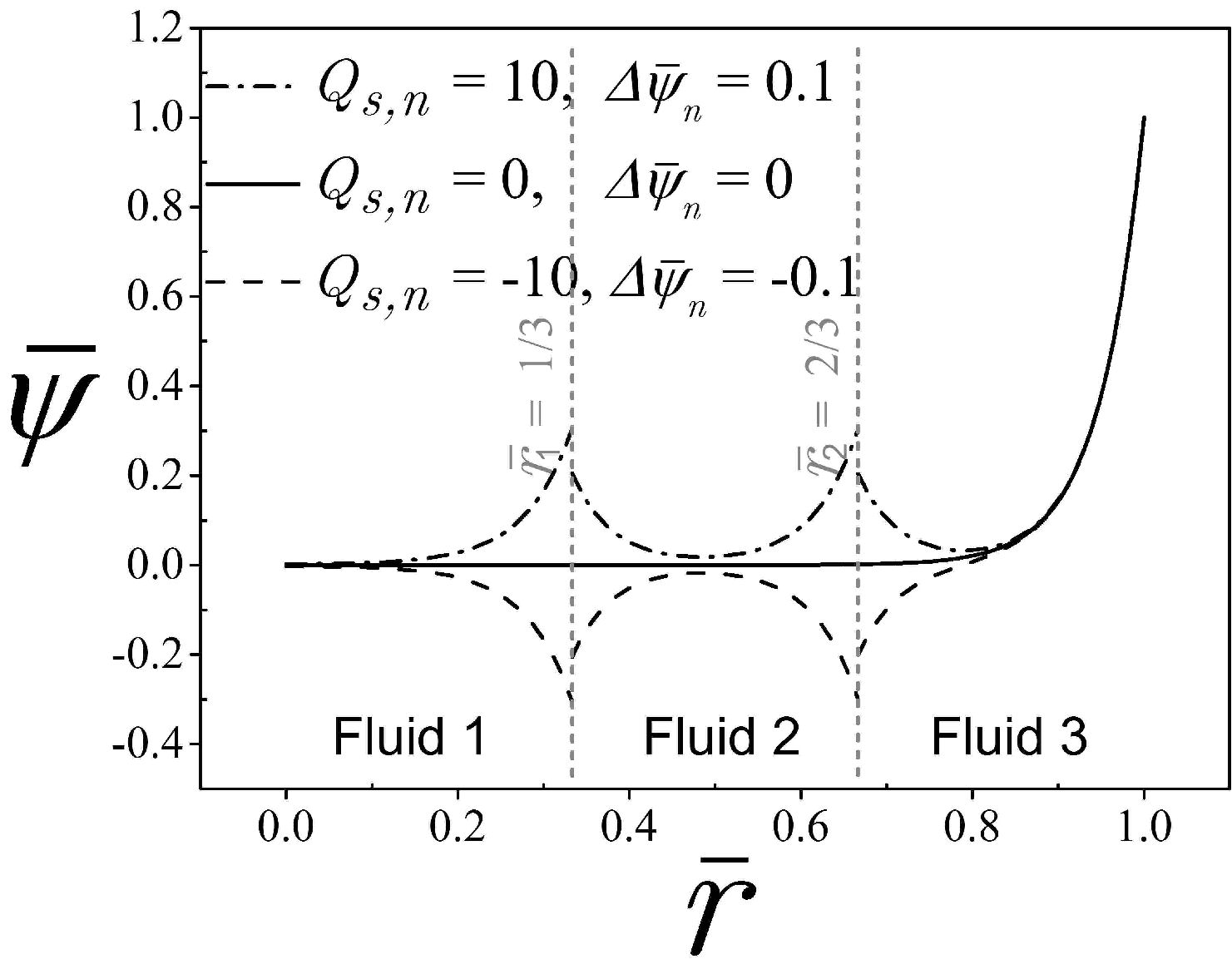
FIGURE 3 Dimensionless electric potential distributions for three immiscible fluids in a capillary with n =3, r¯1=1/3, r¯2=2/3, κ¯n=20, ϵ¯n=1 and different values of Q s,n , and Δψ¯n

Conversely, negative values of Q s,n = −10, yield negative electric potential distributions around each liquid-liquid interface due to the excess of counterions into the electric double layers; while the electric potential discontinuity is maintained via the value of Δψ¯n=-0.1 in the two liquid-liquid interfaces. In the case of null ionic interaction between the immiscible fluids with Q s,n = 0 and Δψ¯n=0, we have that the electric potential has a constant null value from the center of the capillary until increase asymptotically within the electric double layer placed around the solid-liquid interface in fluid 3, to reach their maximum value of ψ¯r¯=1=1 at the wall of the capillary. As can be seen in Fig. 3, all cases for the electric potential distribution overlap in two zones, near to the center of the capillary when r¯0 taking a value of ψ¯=0 and near of the wall of the capillary when r¯1 where ψ¯1.

Figures 4 presents the transient evolution of the dimensionless velocity profiles as a function of the dimensionless radius of a purely electroosmotic flow with Γ = 0, pumping three layers of immiscible fluids. With the aid of the previous results in the electric potential distribution given in Fig. 3, the velocity profiles in Fig. 4(a) corresponds to the condition with Q s,n = 10 and ψ¯n=0.1. Here, because a positive polarity in the electric potential distribution along the cross-section of the capillary and an excess of ions at the liquid-liquid interfaces, the continuity of shear viscous stresses breaks and when the fluids experiment the electroosmotic effects at these interfacial positions producing steep velocity gradients resulting in strong changes in the velocity, in this case in favor of the flow. Also from the mentioned, the velocity profiles in each layer of fluid exhibit a convex shape towards the positive z− direction, converging in each liquid-liquid interface. Conversely, in the case of Fig. 4(c) with Q s,n = −10 and ψ¯n=-0.1, where both by a negative polarity of the electrical potential distribution as an excess of counterions at the liquid-liquid interfaces, produces velocity profiles with a concave shape due to the adverse electroosmotic effects at these interfacial positions; this condition diminishes the magnitude of the velocity profiles regarding Fig. 4(a). While for null ionic interaction between fluid layers with Q s,n = 0 and ψ¯n=0, as is shown in Fig. 4(b), the classic plug-like electroosmotic flow is recovered, and the electroosmotic effects are transmitted outside of the electric double layer placed at the wall of the capillary only by viscous drag to the rest of the fluids. In all cases for velocity, in Fig. 4, the symmetry boundary condition at the centerline of the capillary and the no-slip boundary condition at the wall are accomplished, and the steady-state is reached when t¯. Also, in Figs. 4(a) and 4(c), it is observed that during a period covering the first times in the start-up of the electroosmotic flow, inverse flows are present; for Fig. 4(a) at the time t¯=0.0025, the inverse flow is around the liquidliquid interfaces, while for Fig. 4(c) at t¯=0.04, it is present outside of them.

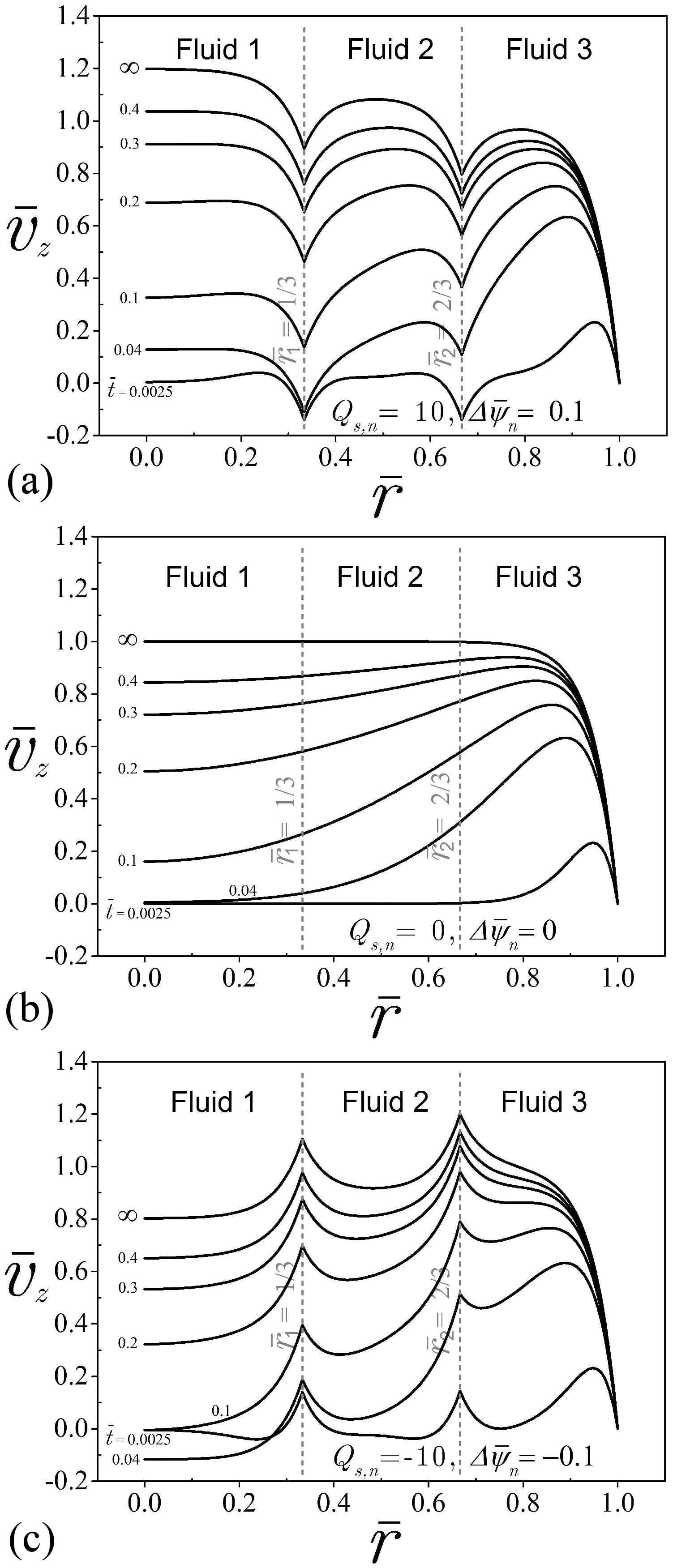
FIGURE 4 Dimensionless velocity profiles of a purely electroosmotic flow for different times with n = 3, r¯1=1/3, r¯2=2/3, κ¯n=20, Γ = 0, ϵ¯n=1, ρ¯n=1 and μ¯n=1. For (a) Q s,n = 10,Δψ¯n=0.1, (b) Q s,n = 0,Δψ¯n=0 and (c) Q s,n =−10,Δψ¯n=-0.1

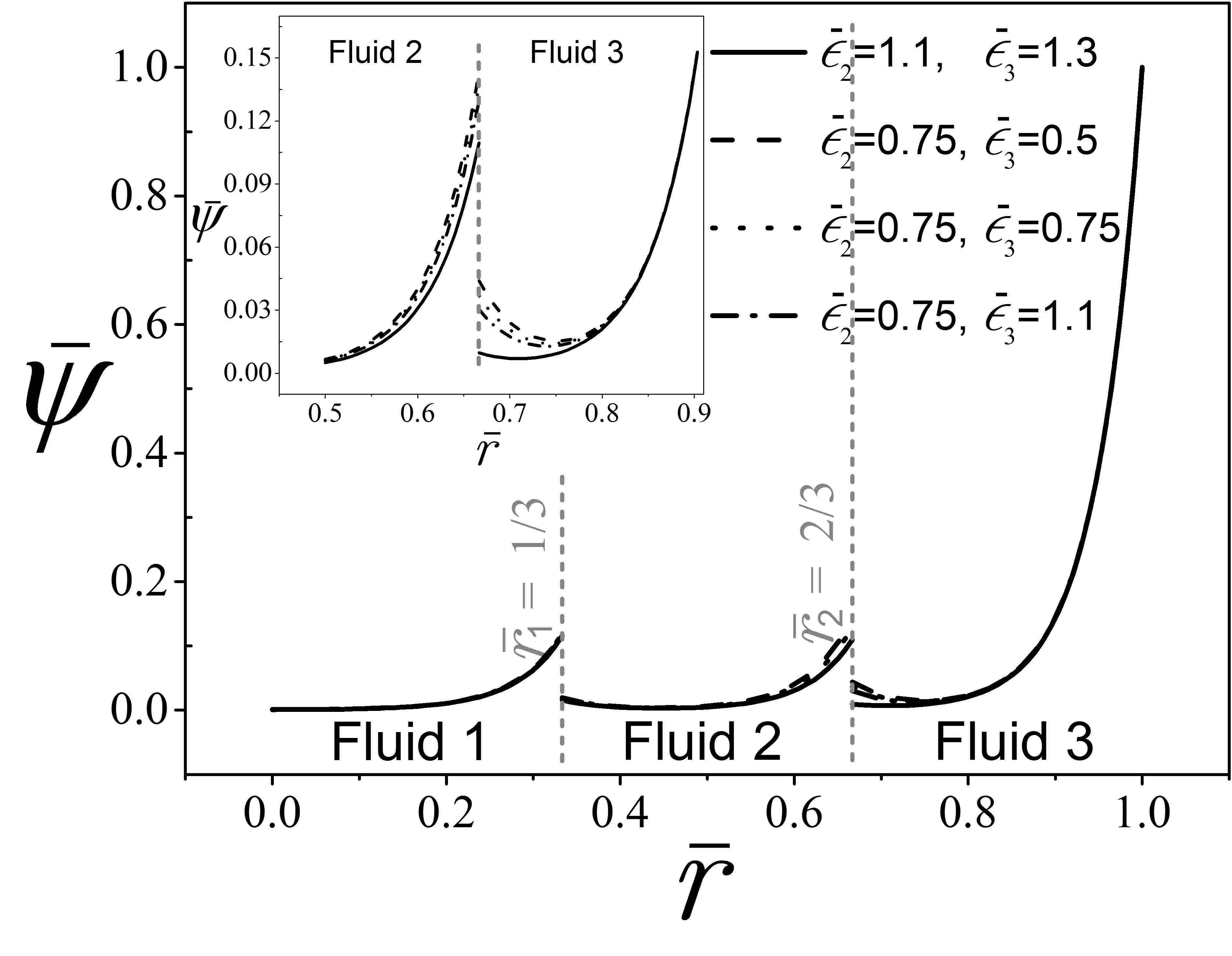
Figure 5 shows the development in the time of dimensionless velocity profiles as a function of the dimensionless radial coordinate of a purely electroosmotic flow of three immiscible fluids, under the influence of the dimensionless dielectric permittivity ratios ϵ¯2 and ϵ¯3, and for the times t¯=0.0025,0.1,0.3 and t¯, respectively. For these results, the dielectric permittivity ratio in fluid layer 1 is maintained constant with ϵ¯1=1 and the other dimensionless parameters selected are in the figure. Since dielectric permittivity is an indicator of the effectiveness or sensitivity of a material to be polarized under an applied external field, in Figs. 5(a)-(d), the velocity profile with greater magnitude corresponds to the case given by ϵ¯2=1.1 and ϵ¯3=1.3, being the combination with the higher values for the dielectric permittivity. In this sense, the velocity profile with smaller magnitude will correspond to the following combination with ϵ¯2=0.75 and ϵ¯3=0.5. On the other hand, by observing Fig. 5(a), it is clear that the effect of the dimensionless dielectric permittivity is stronger in outermost layer, whose velocity grows faster than in the other internal fluids; this effect is extended progressively to the rest of the fluid layers and towards the center of the capillary as time goes, as can be seen in Figs. 5(b) and 5(c), and until the steady-state is reached in Fig. 5(d). The growth of the velocity in fluid 3 is faster compared to the other internal fluids in Fig. 5(a), this is related to the sensitivity in the response of electroosmotic effects into the electric double layers in early times; this response is magnified as the value of dielectric permittivity of the fluid and the magnitude of the electric potential distribution also increase. Therefore, with the aid of Fig. 6 for the electric potential distribution related to Fig. 5, we can see that from any combination of ϵ¯n and ψ¯3 1, the highest values of the electrical potential are obtained in layer 3, in comparison with the rest of layers of fluids. With the mentioned, the largest response of the velocity profile in early times and under the application of an external electric field in the electroosmotic flow is also produced.

FIGURE 5 Dimensionless velocity profiles of a purely electroosmotic flow with n = 3, r¯1=1/3, r¯2=2/3, κ¯n=20, Γ = 0, ρ¯n=1, μ¯n=1, Q s,n =2.5, Δψ¯n=0.1, ϵ¯1=1, and different combinations of ϵ¯2 and ϵ¯2. For (a) t¯=0.0025, (b) t¯=0.1, (c) t¯=0.3 and (d) t¯

FIGURE 6 Dimensionless electric potential distributions for Fig. 5

In Fig. 7 are presented the dimensionless velocity profile of three immiscible fluids as a function of the radial coordinate and time and under different combinations of viscosity ratios μ¯2,3. In all cases, the viscosity ratio for the innermost layer is maintained with a value of μ¯1=1. In Figs. 7(a) to 7(d), the time is increasing from t¯=0.1 until the steady-state when t¯ goes to infinity. Here, we can observe additional characteristics of the multi-layer flow, by following each combination of the viscosity ratios between fluids. The case with μ¯2=1 and μ¯3=5, represents in this group of figures, the case with the greatest resistance to flow because the velocity profile experiment very small changes in their magnitude as the time passes with respect to the other cases. On the contrary case, for the combination of viscosity ratios with μ¯2=10 and μ¯3=0.1, the highest velocity distribution is reached at the end of the transient-state, although this case contains the most viscous intermediate fluid layer with μ¯2=10. With this, it is clear that the influence of the viscosity value in the outermost layer is predominant to define the velocity magnitude along the cross-section of the capillary, more than in some other layer of the inner fluids. However, although the outermost layer is that which define the global magnitude of the velocity profile of the multi-layer flow, the shape of the velocity profile and magnitude in each layer of fluid depend on their viscosity ratio, e.g., by compare the case of the intermediate fluid with μ¯2=1 and the intermediate fluid with μ¯2=0.1, the velocity changes in the first case are small with a flat velocity profile, while in the second case the velocity changes are more representative with prominent parabolic shape.

FIGURE 7 Dimensionless velocity profiles of a purely electroosmotic flow with n = 3, r¯1=1/3, r¯2=2/3, κ¯n=20, Γ = 0, ϵ¯n=1, ρ¯n=1, μ¯1=1, Q s,n =10, Δψ¯n=0.1, and different combinations of μ¯2 and μ¯3. For (a) t¯=0.1, (b) t¯=0.4, (c) t¯=0.9 and (d) t¯

The effect of an external and constant pressure gradient on the flow field via dimensionless parameter Γ, is shown in Fig. 8; therefore, this graph represents the transient evolution of combined electroosmotic-pressure driven flow. The values of Γ = −2 and Γ = 2 show the influence of pressure forces in favor and contrary to the positive z-direction, respectively; the aforementioned can be demonstrated if the velocity profiles under pressure effects are compared in this graph with the case when Γ = 0, for a purely electroosmotic flow. Also, the invariant electric potential at the time is presented in Figs. 8(a)-(c) as dashed lines for Q s,n = 15 and Δψ¯n=0.5; here, the potential slip at the liquid-liquid interfaces and the zeta potential at the solid-liquid interface at the wall, are clear and corresponds with the convex velocity distribution.

FIGURE 8 Dimensionless velocity profiles (solid lines) and electric potential distribution (dashed lines) of a combined electroosmotic-pressure driven flow with n = 3, r¯1=1/3, r¯2=2/3, κ¯n=20, ϵ¯n=1, ρ¯n=1, μ¯n=1, Q s,n = 15, and Δψ¯n=0.5. For (a) Γ=−2, (b) Γ=0 and (c) Γ=2. 

In Fig. 9, the characteristics of a purely electroosmotic flow under the influence of the electrokinetic parameter κ¯n are shown. Regarding the electric potential, in Fig. 9(a), it is observed that as the value of κ¯n=10 increases to the value of κ¯n=50, the electric potential distribution is closer to the capillary wall, while at the interfaces, their distribution is thinner and small in magnitude. The previously mentioned is due to a condition of thinner electric double layers by increase the ionic concentration of the electrolytes or by increasing the radius of the capillary. On the other hand, and based in Fig. 9(b), it is clear that for large values of the electrokinetic parameter with κ¯n=50, the shape of velocity profiles tend to be flat, while for the small values with κ¯n=10, tends to take a parabolic shape when t¯.

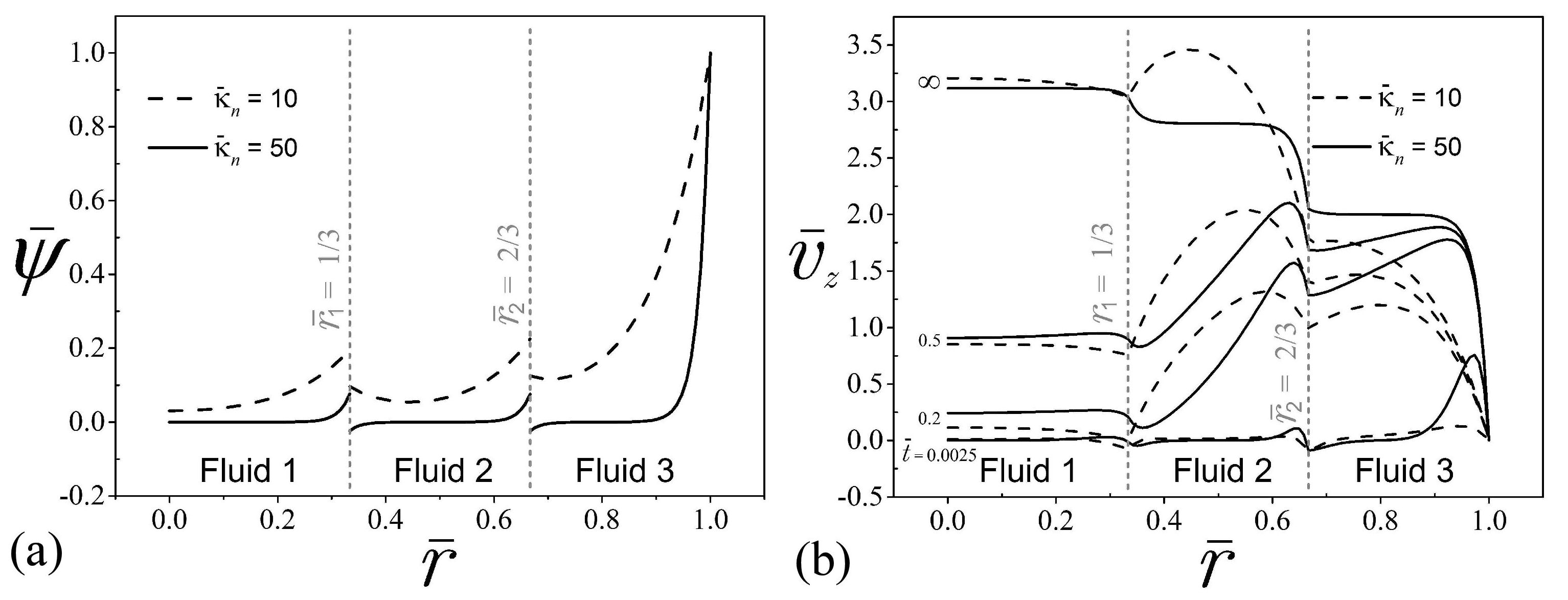
FIGURE 9 (a) Dimensionless electric potential distributions and (b) velocity profiles of a purely electroosmotic flow for four different times with n = 3, r¯1=1/3, r¯2=2/3, Γ = 0, ϵ¯n=1, ρ¯n=1, μ¯1=1, μ¯2=0.1, μ¯3=0.5, Q s,n = 2.5, Δψ¯n=0.1, and two values of κ¯n=10 and κ¯n=50

In Fig. 10, the influence of the dimensionless densities ratios on the velocity profiles during the start-up of purely electroosmotic flow is given. Here, the magnitude of the velocity profile is defined by the heaviness of each layer of fluid, being the lightest fluids that move faster in the flow or vice versa. Therefore, the magnitude of the velocity profile in the transient period of the flow depends on the density ratio value in each layer and their position in the arrangement of the multi-layer flow. It is very clear that when the multilayer electroosmotic flow reaches the steady-state regime in t¯, the heaviness condition disappears, and all velocity profiles overlap. The electric potential distribution for the electroosmotic flow in Fig. 10, can be found in Fig. 9(a).

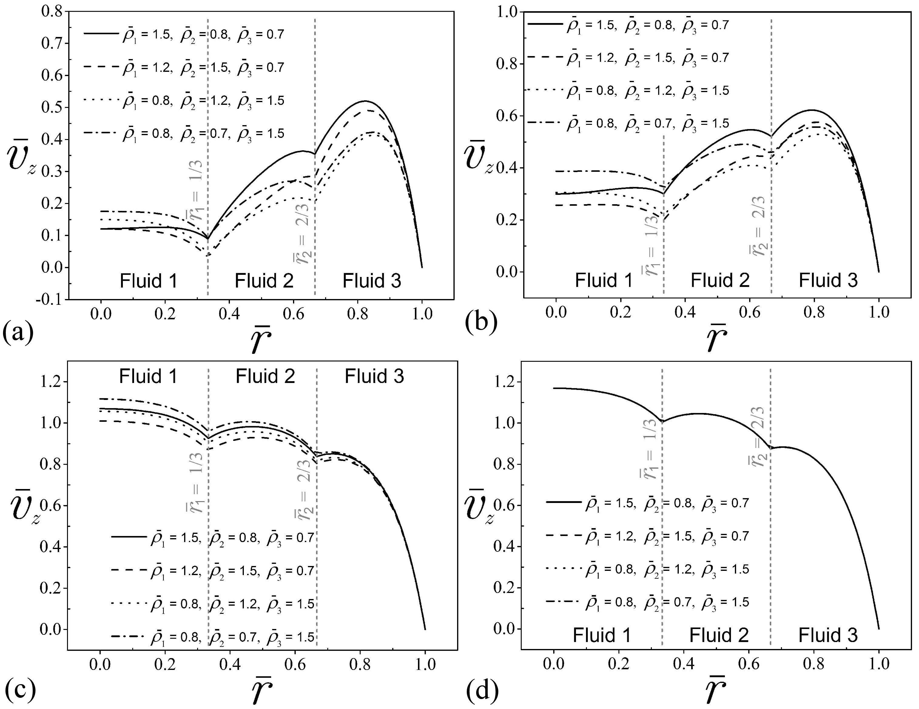
FIGURE 10 Dimensionless velocity profiles of a purely electroosmotic flow with n =3, r¯1=1/3, r¯2=2/3, κ¯n=10, Γ=0, ϵ¯n=1, μ¯n=1, Q s,n =2.5, Δψ¯n=0.1, and different combinations of ρ¯n. (a) t¯=0.05, (b). t¯=0.1, (c) t¯=0.5 and (d) t¯

In Fig. 11, we show the electroosmotic flow of four layers of immiscible fluids with different thicknesses, and a wide combination of all dimensionless parameters studied here. Therefore, we can found interesting combined behaviors on the transient evolution of the velocity profiles, from the early time t¯=0.0025 in Fig. 11(a), to the steady-state in t¯ in Fig. 11(d). Additionally, the corresponding electric potential distributions to generate the electroosmotic flows analyzed in Fig. 11, is given in Fig. 12.

FIGURE 11 Dimensionless velocity profiles of a purely electroosmotic flow with n =4, r¯1=0.1, r¯2=0.4, r¯3=0.8, κ¯1=20, κ¯2=50, κ¯3=10, κ¯4=30, Γ=0, ϵ¯1=1, ϵ¯2=0.8, ϵ¯3=1.1, ϵ¯4=1, ρ¯n=1, Q s,1 =3, Q s,2 =−2, Q s,3 =5, Δψ¯1=0.1, Δψ¯2=-0.25, Δψ¯3=0.2, and different combinations of μ¯n. For (a) t¯=0.0025, (b) t¯=0.05, (c) t¯=0.2 and (d) t¯

FIGURE 12 Dimensionless electric potential distribution for Fig. 11

4.3. Tracking of the velocity

Figure 13 shows the tracking results of the dimensionless velocity as a function of the dimensionless time, evaluated at the centerline of the capillary. This results are taken from the flows presented in Sec. 4.2. For all cases, we can see a gradual increase in the velocity as the time progresses since the rest to reach the steady-state. It is clear from Figs. 13(a), (b), (d)-(f), that the time to reach the steady-state of the fluid flows is independent of the dimensionless parameters Q s,n , ψ-n, -n, Γ, κ-n, and ρ-n, respectively; however, it is strongly dependent of the viscosity ratios µ-n as is shown in Fig. 13(c). Again, the accuracy of our solution was validated in Fig. 13(a) for Q s,n = 0 and ψ-n=0, with the aid of the solution reported by Keh and Tseng [11] for a single fluid.

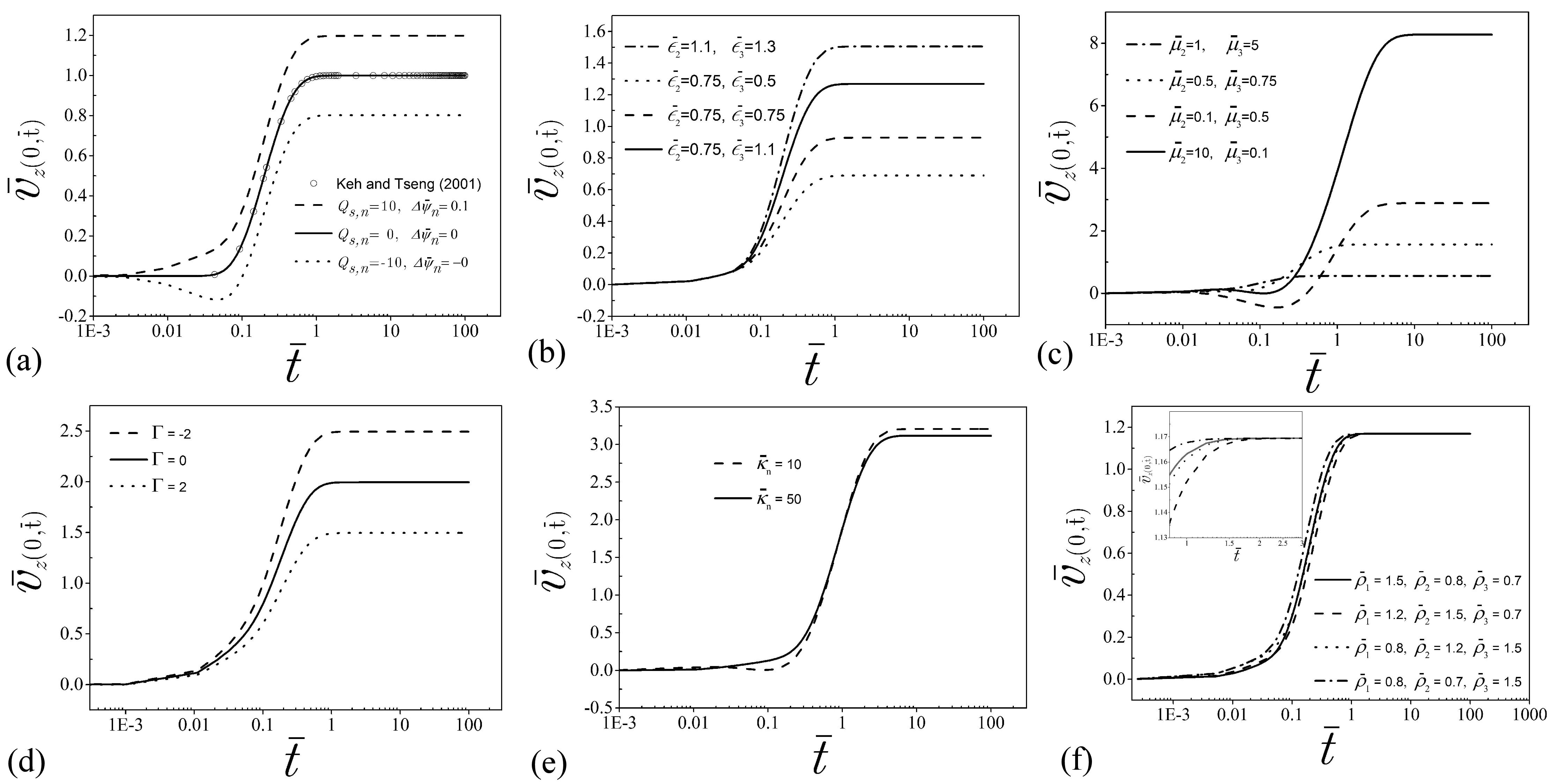
FIGURE 13 Tracking of the velocity in the multi-layer flow as a function of the dimensionless time evaluated at the centerline of the capillary. (a) effect of Q s,n and Δψ¯n (from Fig. 4), (b) effect of ϵ¯n (from Fig. 5), (c) effect of μ¯n (from Fig. 7), (d) effect of Γ (from Fig. 8), (e) effect of κ¯n (from Fig. 9) and (f) effect of ρ¯n (from Fig. 10). 

5. Conclusions

In the present work, we realize a semi-analytical solution of the start-up of combined electroosmotic and pressure driven flow of multi-layer immiscible fluids within a narrow capillary. The parametric study is based on the different fluid properties, geometrical characteristics, and boundary conditions in the solid-liquid and liquid-liquid interfaces. Considering the studied flow conditions was demonstrated that the presence of electric double layers at liquid-liquid interfaces break the continuity of the electric potential distribution and the shear viscous stresses, producing representative changes of the velocity distributions, which could be in favor or against of the flow. In other results, it was determined that the physical and electric properties of the outermost layer of the multi-layer flow, make it govern the global magnitude of the velocity distribution over the cross-section of the capillary. On the other hand, the time to reach the steady-state regime of the fluid flows is strongly controlled by the viscosity ratios, and it is independent of the other dimensionless parameters presented here. Therefore, this investigation is an important theoretical contribution to simulate transient multi-layer fluid flows under electric interfacial effects, covering different implications that emerge in the design of small devices into the chemical, biological and clinical areas.

Finally, several implications can to be analyzed. For example, it is recommended to address the following issues to extend the present work: the analysis can include non-Newtonian fluids, treat the liquid-liquid interfaces as perturbed lines or with shape defects, and also, the interfaces can be treated as transitional layers with non-zero thickness, where two phases partly dissolve in each other, and the properties of the medium gradually change from the properties of one phase to the other.

Acknowledgments

This work was supported by the Instituto Politécnico Nacional in Mexico (grant number SIP-20195892).

References

1. S. Badilescu and M. Packirisamy, BioMEMS Science and Engineering Perspertives. CRC Press and Taylor & Francis Group, Boca Raton, FL, U.S., (2011). [ Links ]

2. E. Meng, Biomedical Microsystems. CRC Press and Taylor & Francis Group, Boca Raton, FL, U.S., (2010). [ Links ]

3. C. Kleinstreuer, Microfluidics and Nanofluidics. Theory and Selected Applications. Wiley, Hoboken, NJ, U.S., (2014). [ Links ]

4. A. Ramos, Electrohydrodynamic and magnetohydrodynamic micropumps. In Microfluidic Technologies for Miniaturized Analysis Systems; Hardt, S., Schönfeld, F., Eds.; Springer, Boston, MA, U.S., (2007). [ Links ]

5. D.J. Laser and Santiago J.G., J. Micromech. Microeng. 14 (2004) R35-R64. [ Links ]

6. D. Li, Encyclopedia of Microfluidics and Nanofluidics. Springer, Boston, MA, U.S., (2008). [ Links ]

7. J. Friend and L.Y. Yeo, Rev. Mod. Phys. 83 (2011) 647-704. [ Links ]

8. C. Zhang, J. Xu, W. Ma and W. Zheng, Biotechnol. Adv. 24 (2006) 243-284. [ Links ]

9. J.H. Masliyah and S. Bhattacharjee, Electrokinetic and Colloid Transport Phenomena. Wiley-Interscience, Hoboken, NJ, U.S., (2006). [ Links ]

10. C.L. Rice and R. Whitehead, J. Phys. Chem. 69 (1965) 4017- 4024. [ Links ]

11. H.J. Keh and H.C. Tseng, J. Colloid Interface Sci. 242 (2001) 450-459. [ Links ]

12. S. Wang and M. Zhao, Eur. J. Mech. B: Fluids 54 (2015) 82-86. [ Links ]

13. H.-K. Tsao, J. Colloid Interface Sci. 225 (2000) 247-250. [ Links ]

14. R. Na, Y. Jian, L. Chang, J. Su and Q. Liu, Open J. Fluid Dyn. 3 (2013) 50-56. [ Links ]

15. L.L. Ferrás, A.M. Afonso, M.A. Alves, J.M. Nóbrega and F.T. Pinho, J. Colloid Interface Sci. 420 (2014) 152-157. [ Links ]

16. C. Yang, C.B. Ng and V. Chan, J. Colloid Interface Sci. 248 (2002) 524-527. [ Links ]

17. J. Escandon, E. Jiménez, C. Hernández, O. Bautista and F. Méndez, Eur. J. Mech. B: Fluids 53 (2015) 180-189. [ Links ]

18. A.M. Afonso, M.A. Alves and F.T. Pinho, J. Non-Newton. Fluid Mech. 159 (2009) 50-63. [ Links ]

19. A. Miller, A. Villegas and F.J. Diez, Electrophoresis 36 (2015) 692-702. [ Links ]

20. A. Sadeghi, M. Azari and S. Chakraborty, Int. J. Therm. Sci. 122 (2017) 162-171. [ Links ]

21. X. Yang, H. Qi and X. Jiang, Appl. Math. Lett. 78 (2018) 1-8. [ Links ]

22. M. Liu, Y. Liu, Q. Guo and J. Yang, J. Electroanal. Chem. 636 (2009) 86-92. [ Links ]

23. S. Movahed, S. Khani, J.Z. Wen and D. Li, J. Colloid Interface Sci. 372 (2012) 207-211. [ Links ]

24. A.J. Moghadam, Int. J. Eng. Trans. A: Basics 29 (2016) 1469-1477. [ Links ]

25. A. Matías, F. Méndez and O. Bautista, Micromachines 8 (2017) 232. [ Links ]

26. Y. Huang, H. Li, and T.N. Wong, Int. J. Heat Mass Transf. 74 (2014) 368-375. [ Links ]

27. A.M. Afonso, M.A. Alves and F.T. Pinho, J. Colloid Interface Sci. 395 (2013) 277-286. [ Links ]

28. Y. Gao, C. Wang, T.N. Wong, C. Yang, N.-T. Nguyen and K.T. Ooi, J. Micromech. Microeng. 17 (2007) 358-366. [ Links ]

29. Y. Gao, T.N. Wong, C. Yang and K.T. Ooi, Colloid Surf. APhysicochem. Eng. Asp. 266 (2005) 117-128. [ Links ]

30. A.G. Volkov, D.W. Deamer, D.L. Tanelian and V.S. Markin, Colloid Prog. Surf. Sci. 53 (1996) 1-134. [ Links ]

31. T. Wandlowsky, K. Holub, V. Mareček and Z. Samec, Electrochim. Acta 40 (1995) 2887-2895. [ Links ]

32. Z. Samec, V. Mareček and D. Homolka, J. Electroanal. Chem. 187 (1985) 31-51. [ Links ]

33. Q. Cui, G. Zhu and E. Wang, J. Electroanal. Chem. 383 (1995) 7-12. [ Links ]

34. W. Choi, A. Sharma, S. Qian, G. Lim and S.W. Joo, J. Colloid Interface Sci. 357 (2011) 521-526. [ Links ]

35. J. Su, Y.-J. Jian, L. Chang and Q.-S. Liu, Acta Mech. Sin. 29 (2013) 534-542. [ Links ]

36. Y. Jian, J. Su, L. Chang, Q. Liu and G. He, Z. Angew. Math. Phys. 65 (2014) 435-447. [ Links ]

37. G.C. Shit, A. Mondal, A. Sinha and P.K. Kundu, Colloid Surf. A-Physicochem. Eng. Asp. 506 (2016) 535-549. [ Links ]

38. L. Haiwang, T.N. Wong and N.-T. Nguyen, Int. J. Heat Mass Transf. 53 (2010) 772-785. [ Links ]

39. J. Li, P.S. Sheeran and C. Kleinstreuer, J. Fluids Eng.-Trans. ASME 133 (2011) 111202. [ Links ]

40. Y. Gao, T.N. Wong, C. Yang and K.T. Ooi, J. Colloid Interface Sci. 284 (2005) 306-314. [ Links ]

41 -C.-H. Chen, J. Heat Trans.-T. ASME 131 (2009) 022401. [ Links ]

42. K. Horiuchi, P. Dutta and A. Hossain, J. Eng. Math. 54 (2006) 159-180. [ Links ]

43. X. Xuan, B. Xu, D. Sinton and D. Li, Lab Chip 4 (2004) 230- 236. [ Links ]

44. G.D. Ngoma and F. Erchiqui, J. Micromech. Microeng. 16 (2006) 83-91. [ Links ]

45. H.-L. Zhang and S.-J. Han, J. Chem. Eng. Data 41 (1996) 516-502. [ Links ]

46. S. Levine, J.R. Marriott, G. Neale and N. Epstein, J. Colloid Interface Sci. 52 (1975) 136-149. [ Links ]

47. R.F. Probstein, Physicochemical Hydrodynamics: An introduction. Wiley-Interscience, Hoboken, NJ, U.S., (2003). [ Links ]

48. J.D. Hoffman, Numerical Methods for Engineers and Scientists. Marcel Dekker, Inc., NY, U.S., (2001). [ Links ]

49. J. Abate and W. Whitt, Informs J. Comput. 18 (2006) 408-421. [ Links ]

Received: July 27, 2019; Accepted: October 18, 2019

∗e-mail: jescandon@ipn.mx

Creative Commons License This is an open-access article distributed under the terms of the Creative Commons Attribution License