1.Introduction

This paper analyzes the Trajectory Tracking for a Fractional Order Nonlinear System for a Fractional Order Time-Delay Neural Network, which is forced to follow a Fractional Order Reference signal generated by a nonlinear chaotic system. The control law that guarantees trajectory tracking is obtained by using the Fractional Order Lyapunov-Krasovskii and Lur’e methodology Chaotic behavior, as a characteristic of a dynamical system, could be desirable or undesired, depending on the current application. In mixing substances process, a chaotic behavior might improve the efficiency of the system, while in the process which involves vibrations, chaos could produce critical structural failures. As a consequence, it is important to be able to manipulate the chaotic nature of the system, driving a stable system to be chaotic or otherwise stabilize a chaotic system. In many applications, it is also important to change the chaotic nature of a system without losing the chaotic behavior. Controlling and synchronizing chaotic dynamical systems has recently attracted a great deal of attention within the engineering society, in which different techniques have been proposed. For instance, linear state space feedback, Lyapunov-Krasovskii function methods ¹, adaptive control ². Using the inverse optimal control approach, a control law ³, which allows reproducing chaos on a Dynamical Neural Network, was discussed in (4). We further extend these results to the Fractional Order Time-Delay Neural Networks case for nonlinear system trajectory tracking. The proposed new scheme is composed of a Fractional Order delayed dynamical neural identifier, which builds an on-line model for the unknown delayed neural network, and control law.

There are several ways of defining the derivative and fractional integral, for example, the derivative of Grunwald-Letnikov given by Eq. (1)

Where □ is a flooring-operator while the RL definition is given by:

For (n-1 < α < n) and Γ(x) is the well-known Euler’s Gamma function

Similarly, the notation used in ordinary differential equations, we will use the following notation, Eq. (3), when we are referring to the fractional-order differential equations where, α k ϵ □ + .

Which is:

The Caputo´s definition can be written as

For (n-1 < α < n)

Trajectory tracking, synchronization, and control of linear and nonlinear systems are a very important problem in science and control engineering. In this paper, we will extend these concepts to force the nonlinear system (Fractional Order Delayed Plant) to follow any linear and nonlinear Fractional reference signals generated by fractional order differential equations.

This obtained result, modeling by differential equations of fractional order, is new, unlike other results obtained by the authors, modeled by ordinary differential edifications.

The effectiveness of the methodologies, from our point of view, are equal, the difference is that we have observed that the response of the controller is in smaller magnitude in the systems of fractional order than in the systems of ordinary differential equations, and also, in the systems of fractional order have some slack by varying the order of the fractional system, which causes the response of the system to be smoother, which does not happen with ordinary non-linear systems.

The applicability of the approach is illustrated by one example: chaos synchronization. In the following, we first briefly describe the dynamic of the fractional order Time-Delay Neural Network to be used.

2. Mathematical models

The differential equation will be modeled by the neural network ⁵:

where τ is the fixed known time delay, x is the state, u is the input, A = −λI, with λ being a positive constant, W is the state-feedback matrix, and σ(∗) = tan h(∗) is a Lipschitz function ⁶ such that σ(x)=0 only at x =0, with Lipschitz constant L_σ. It is clear that x =0 is an equilibrium point of this system, when u =0.

The system, to be tracked by the neural network, is defined as:

Where aDtaaxr is the state, u_r is the input, f(∗) and g(∗) are smooth nonlinear functions of appropriate dimensions.

As is clear, this is very general, and the model (6) can be complex such as chaotic nonlinear system.

3. Trajectory tracking

The objective is to develop a control law such that the delayed neural network (5) tracks the trajectory of the dynamical sys tem (6). We dene the tracking error as e = x − x _r , whose derivative for time is:

Substituting (5) and (6) in (7), we obtain

aDtae=Ax+Wσxt-τ+u-fxr-gxrur

Adding and subtracting to (8) the terms W_σ[x_r(t − τ)] and α(t), we have

Where α(∗) is a function to be determined. For system (5) to follow model (6), the following solvability assumption is needed, as discussed in ⁷:

Assumption 1. There exist functions ρ(t) and α(t), such that

ρ(t)= xr(t). (10) It follows from (10) and (6) that

So that (9) becomes

aDtae=Ae+W(σxt-τ-σxrt-τ+u-a(t))

Let’s define u~=(u-a(t)

It is clear that e = 0, is an equilibrium point of (12), when u~=0. In this way, the tracking problem can be restated as a global asymptotic stabilization problem for the system (12).

4. Tracking error stabilization and control design

To establish the convergence of (12) to e = 0, which ensures the desired tracking, .rst, we propose the following Krasovskii ⁸ and Lur’e functional ⁹. This is essential for the design of a globally and asymptotically stabilizing control law. We select

The time derivative of (13), along the trajectories of (12)

We select ϕσTt-τ=σx(t-τ)-σxrt-τ

Next, let consider the following inequality, proved in ¹⁰:

which holds for all matrices X, Y ∈ Rnxk and Λ ∈ Rnxn with Λ=Λ^T > 0. Applying (17) with Λ= I to the term ϕe,xrTWϕσT(t-τ), we get

By simplifying (18), we obtain

Since φ(e, x_r) is a sector function for e, there exist positive constants k₁ and k₂ such that k1e22≤ϕe,xrT≤k2e22 ¹¹. Also, since φ(e, x_r) is Lipschitz for e, there exist a positive constant L_σ such that ϕe,xrTϕe,xr≤Lσ2222. Henceforth (19) can be rewritten and then we have that

By simplifying (20), we have

Since φ_σ is Lipschitz with Lipschitz constant L_σ¹², then

Applying to ϕσT(t)WTWϕσ(t)

With Lσ2 the Lipschitz constant of (23) σ(∗). To the right hand, third term of (17), we obtain:

Now, we suggest to use the following control law:

Where β is a positive constant and (R(e))⁻¹ is a function of e. At this point, substituting (25) into (24), we obtain

Then aDtaV(e)<0 for all e ≠ 0. This means that the proposed control law (27) can globally and asymptotically stabilize the error system, therefore ensuring the tracking of (5) by (6).

Finally, the control action driving the recurrent neural net works is given by:

We summarize the above developed analysis in the following Theorem.

Theorem 1. The control law (27) ensures that the Time-Delay Neural Network (5) tracks the reference system (6).

5. Simulations

To illustrate the applicability of the discussed results, we selected, the following delayed neural network: aDtaxp=Ax+Wσx(t-τ)u where

The reference signal, which the neural network has to fol low is the chaotic circuit of Chua ¹³, described by the differential equation of fractional order:

aDtayr=xr-yr-zr

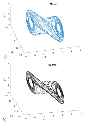
FIGURE 1 α =1 Simulation result for the Non-Linear System and the Reference Signal synchronization between the delayed neural network and the Chua.s circuits. The Non-linear system is coupled to the slave system with the first state variable and delay (τ = 15 t Sec): Three-dimensional view on the double scroll attractor generated for a) Non-Linear System (master system) and b) Reference Signal (slave system). 

The following simulations were performed applying Mat-Lab / Simulink, using the fourth order Runge Kutta method.

The experiment is performed as follows. Both systems, the delayed neural network, and the Chua’s circuits, evolve independently until τ = 15 seconds: at that time, the proposed control law (23) is incepted.

For 15 seconds, the non-linear system is in open loop (Without Control), later, passing that time delay, the control is applied, and the trajectory tracking objective is performed, as can be seen in Fig. 2, 3, and 4, and the tracking errors tend to zero after the controller goes into operation.

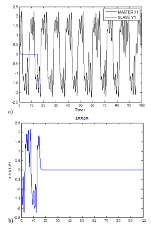
FIGURE 2 Time evolution for Delayed Neural Network and Chua’s circuits with initial condition (0.7; 0; 0) and the error signal (x₁(t) − y₁(t)) for time. 

FIGURE 3 Time evolution for Delayed Neural Network and Chua’s circuits with initial condition (0.7; 0; 0) and the error signal (x₂(t)−y₂(t))concerning time. 

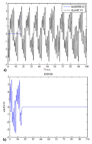
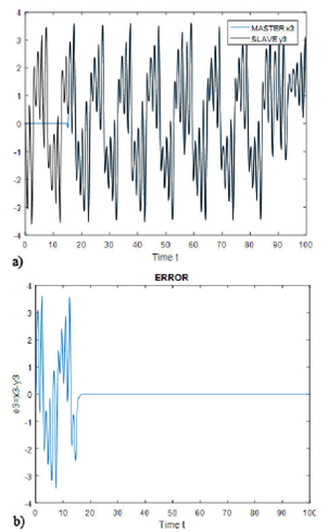
FIGURE 4 Time evolution for Delayed Neural Network and Chua’s circuits with initial condition (0.7; 0; 0) and the error signal (x₃(t)−y₃(t))concerning time. 

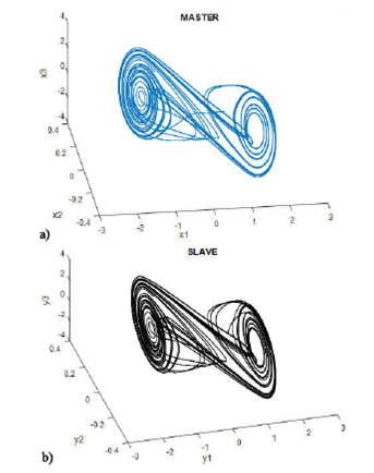
FIGURE 5 α =0.00001 Simulation result for master-slave synchronization between the fractional-order delayed neural network and the Chua’s circuits. The master system is coupled to the slave system with the first state variable and delay (τ = 15 Sec): Three-dimensional view on the double scroll attractor generated for a) master system and b) slave system. 

The experiment is performed as follows. Both systems, the fractional-order delayed neural network and the Chua.s circuits evolve independently until τ = 15 seconds: at that time, the proposed control law (23) is incepted. Simulation results are presented in Fig. 6, 7, 8, for state 1, state 2 and state 3, respectively. As can be seen, tracking is successfully achieved.

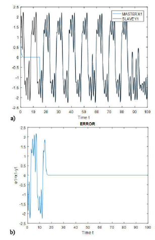
FIGURE 6 Time evolution for the Fractional Order Delayed Neural Network and Chua’s circuits with initial condition (0.7; 0; 0) and the error signal (x₁(t) − y₁(t)) concerning time. 

FIGURE 7 Time evolution for the Fractional Order Delayed Neural Network and Chua’s circuits with initial condition (0.7; 0; 0) and the error signal (x₂(t) − y₂(t)) concerning time. 

FIGURE 8 Time evolution for the Fractional Order Delayed Neural Network and Chua’s circuits with initial condition (0.7; 0; 0) and the error signal (x₃(t) − y₃(t)) concerning time. 

6. Conclusions

We have presented the controller design for trajectory tracking determined by a Fractional Order Time-Delay dynamical network. This framework is based on dynamic Fractional Order delayed neural networks, and the methodology is based on Fractional Order Lyapunov-Krasovskii and Lur’e theory. The proposed Inverse Optimal Control Law is applied to a dynamical fractional order delayed neural network and the Chua’s circuits, respectively, being able to also stabilize in asymptotic form the tracking error between two systems. The results of the simulation show clearly the desired tracking.

In future work, it can be mentioned that the results will be extended to model non-linear systems, whose mathematical model is not completely known, and in that sense, it can be decided that the laws of control and laws of learning are robust.

It is important to mention that, we will are work on simulation in real time to control a humanoid, and these results are very promising, since they would help people who have lost some lower limb, and to control humanoids, which could help in tasks that are dangerous for humans.