


 text new page (beta)
 English (pdf)
 Article in xml format
 Article references
 Send this article by e-mail
 Cited by SciELO
  Similars in
SciELO
Similars in
SciELO 
 Permalink
1.Introduction
During the past decade, a variety of nuclear phenomena like magnetic rotation 1, chiral twin bands 2, shape coexistence 3,4, superheavy elements (5) and superdeformation 6 have been observed, which originate from single-particle and collective motion as well as their interplay. Traditionally, Strutinsky’s shell correction method 7 has been one of the central approaches for calculation of potential energy surfaces 8,9,2, which is a key to understand these phenomena. This method, also known as the macroscopic plus microscopic approach, obtains the fluctuating part of the level density (the shell correction term) arising from the quantal shell correction energy. Parallel to Strutinsk’s method, semiclassical methods have been developed 10-12, which can explain successfully the features of both ordered and chaotic quantum systems. Recently, the mixing of deuteron states (3 S 1 and 3 D 1 ) with tensor interaction has been semiclassically analyzed 13.
One such semiclassical technique, known as periodic orbit theory (POT), was initiated nearly four decades ago by Gutzwiller 10, it has emerged as one of the most powerful methods of understanding the quantum spectra. Semiclassical trace formula, the as developed by Gutzwiller (14) for the fluctuating part of level density of a quantum system is given by
The left-hand side of Eq. (1) is a quantum mechanical quantity, whereas the right-hand side contains only the classical quantities. Here, T
PPO
represents the time period of the primitive periodic orbit, and
Subsequently, several extensions of Gutzwiller’s semiclassical trace formula were made to include regular and mixed dynamics for explaining quantum shell effects in many physical systems 15-18. One such generalization was reported by Strutinsky et al. 19 to systems with continuous symmetries by explicitly taking into account the degeneracy of the classical orbits. This method was successfully applied to phenomenological potentials used in nuclear physics 19, yielding a semiclassical interpretation of ground-state deformation as a function of particle number. One of us 20 has also obtained an eigenvalue spectrum for a particle enclosed in an infinitely high spheroidal cavity by using the formalism of Strutinsky et al. On comparing this semiclassical eigenvalue spectrum with corresponding quantum mechanical values 21, we have established the importance and significant contribution of planar (both in the axis of symmetry plane and the equatorial plane) and 3-dimensional orbits for the normal deformed and the superdeformed regions. Further, this semiclassical method has been extended 22 to explain elegantly the mass asymmetry in nuclear fission 23.
Amann and Brack 24 have developed trace formula for a nuclear system in a 3-dimensional harmonic oscillator mean-field with a spin-orbit interaction of Thomas type. In the strong coupling limit, singularities occur in phase space where the spin-orbit interaction locally becomes zero. These singularities impose severe restrictions on the applicability of the trace formula. However, they have pointed out that the leading orbits with shortest periods are free from singularities and lead to excellent results for the coarse-grained level density, as long as bifurcations of these orbits are avoided.
It is worthwhile to mention here that Littlejohn and Flynn25 developed a semiclassical theory of systems with multi-component wavefunctions and applied 26 it to the WKB quantization of integrable spherical systems with the standard spin-orbit interactions. Frisk and Guhr 27 have studied the deformed systems with spin-orbit interaction by approximating the Schrodinger equation semiclassically. Here, the information about the periodic orbits is extracted from the Fourier transform of the quantum mechanical spectra.
The present work aims to obtain the complete spectrum for a particle moving in an isotropic three-dimensional harmonic oscillator mean-field with spin-orbit interaction. This work is based on the formalism developed by Strutinsky et al. 19. The semiclassical interpretation for a nucleon in an isotropic oscillator mean-field was first given by Bohr and Mottelson 28. They pointed out that only the pendulating orbits (also known as diametric orbits) are possible in this potential. These orbits are traced by a particle by executing two radial oscillations for each angular motion (i.e. (ω r /ω θ = 1/2). Such a trajectory coincides with l= 0 axis. We will show that our periodicity condition confirms their observation, and the calculated eigenvalue spectrum is exactly in agreement with a quantum mechanical one.
Further, the effect of spin-orbit coupling in the mean-field arises only if there is a contribution of orbits with l≥ 0. Such trajectories are obtained in our trace formula by putting the constraint that the particle is reflected at r=R 0 (R 0 being the nuclear radius), instead of infinity. This is an ideal situation for the nuclear shell model, which states that a particle moving in harmonic oscillator mean-field is confined in a spherical cavity of radius R 0 . In this work, we have fixed the potential strength with the help of virial theorem. The complete formalism is free from singularities and does not involve any fitting parameter.
A complete trace formula for a particle moving in a three-dimensional harmonic isotropic oscillator mean-field with spin-orbit coupling is given in Sec. 2. Section 3 is devoted to results and discussion. The conclusions are summarized in Sec. 4.
2.Trace formula for isotropic harmonic oscillator mean-field with spin-orbit coupling
For the bound states of a single particle Hamiltonian H, the level density is generally defined as a sum of Dirac delta distributions,
This sum runs over all the eigen-energies E i (including degeneracies). It can split into a smooth and an oscillating part:
The oscillating component of the single particle level density δg(E), in cylindrical coordinates (ρ,ϕ,z) is given by
The factor f β,m equals to 1 for the diametric orbits and 2 for other orbits like triangles, squares, etc. The time-period for the path from the initial point FORMULA to the final point FORMULA for energy E is defined as
The quantity J in Eq. (4) is the Jacobian of transformation between two sets of classical quantities (p ρ ,P z ,t β,m ) and (ρ′,z′,E), which are related by the classical equations of motion. Here, β denotes the type of orbits and m is the number of reoetitions of a given type of orbit.
The periodic orbit sum in Eq. (4) does not converge in most cases. Since the maximum contribution to the gross shell structure comes from the shortest periodic orbits. It has now become customary to carry out a smooth truncation of the contributions of the longer periodic orbits by folding the level density with a Gaussian function 12 of width γ,
The averaging width γ is chosen to be larger than the mean spacing between the energy levels within a shell, but much smaller than the distance between the gross shells. This averaging ensures that all longer paths are strongly damped and only the shortest periodic orbits contribute to the oscillating part of the level density. Also, the effect of degeneracies is included in Eq. (4) by using the prescription outlined in Ref. 19.
We have approximated the nuclear mean-field by an isotropic harmonic oscillator. The Hamiltonian for a single particle of mass M is expressed in terms of spherical polar coordinates (r,θ,ϕ) and the conjugate momenta (p r ,p θ ,p ϕ ) as
Equation (7) leads to a Hamilton-Jacobi equation, which can be solved by using the separation of variable technique. Therefore, the classical dynamics of a particle is determined by the following three partial actions:
Here, ε and l z are the separation constants and are obtained from the following periodicity conditions.
The integration in the r-coordinate of Eq. (9) is obtained analytically under two limiting approximations: (i) the upper limit lies at infinity and (ii) it lies at R 0 . Both these cases are discussed in the following subsections.
2.1.Case I: upper bound lies at infinity
The limits of radial integration are determined by the reflection points which, in turn, are obtained by solving the equation
Since the radial coordinate is positive, so we consider the following positive roots of equation (13) for the lower and upper limits of the integration in Eq. (4.9).
with σ 2 =ε / (E/ω)2, a dimensionless constant. Thus the action in the radial coordinate becomes
The first periodicity condition Eq. (11) implies ω r = 2ω θ , i.e., only the pendulating orbits are possible, which confirms the result of Bohr and Mottelson 28. The second condition fixes ω θ =ω ϕ . These constraints clearly indicate that both separation constants ε and l z are constants of motion.
Thus the total action in Eq. (4) is obtained as
The Maslov index α β,m in Eq. (4), plays a very crucial role in the periodic sum as it decides the relative phase of the various terms in the summation. Following Creagh and Littlejohn 29 and Brack and Bhaduri 12, we obtain the following Maslov indices for the pendulating orbits.
Finally, the Jacobian in Eq. (4) is calculated numerically using the procedure outlined in Ref. 20. The calculations of Jacobian involve the generalized radial, and axial coordinates ρ, z respectively and their generalized momenta. These generalized coordinates are defined as :
The corresponding canonically conjugate momenta p ρ and p z are
These quantities are inserted in Eq. (4) to calculate the fluctuating part of the level density.
The smooth part of the density of states is calculated within the Thomas-Fermi approximation and is given by
The Eq. (22) has already been multiplied by a factor of 2 to include the spin degeneracy. For the harmonic oscillator potential, V= (1/2)mω
2
r
2
, the integral is evaluated analytically, and we obtain
The harmonic potential with asymptotic reflection point at infinity generates only the pendulating trajectory (i.e. l= 0. A significant contribution of
2.2.Case II: The upper reflection point at R 0
In this case, the particle motion is bounded between an upper limit provided by the radius of sphere r=R 0 and a lower limit fixed at r min (see Eq. (14)). It is worthwhile to mention here that such a scenario corresponds to a particle enclosed in a spherical cavity with perfectly reflecting walls. The radial action, given by Eq. (9), becomes:
Here, σ 1 = (Mω 2 R 0 2)/2E is a dimensionless constant and refers to potential strength. Another dimensionless constant σ 2 =ε 2 /(2MER 0 2) is related to the separation constant ε and is fixed by the periodicity condition Eq. (11) as
The periodicity condition Eq. (12) gives ω θ =ω ϕ , which implies that l z is again a constant of the motion. This gives us the trajectories with l≥ 0. The constant, σ 1 is fixed by using the virial theorem as discussed below.
We know that
Here, the bar on the physical quantities T and V refer to an average over a single period of motion. Thus the total action in (4) is obtained as
The Maslov index α β,m , in this case, is given by the following expressions:
For diametric orbits (l= 0 trajectories),
For other orbits (l= 0 trajectories),
Here, also the Jacobian is calculated by using the procedure as discussed in case I.
Next, the maximum limit for the repetition parameter m in Eq. (4) is obtained by considering that the longest periodic orbit, out of the permissible families β, traverses only once in the cavity. This fixes the repetition numbers of the individual families concerning that of the largest one, i.e.
The length of the orbit L β , is related to the action S β by the relation
Thus, the fluctuating part of the level density is fully established by including all the above mentioned terms in Eq. (4).
Finally, the smooth part is obtained by using the spherical cavity considerations 30
where, V, S, and C refer to the volume, surface area, and radius of curvature of the spherical cavity, respectively.
2.3.Inclusion of
The Hamiltonian, H, in Eq. (7) is modified by including the
This equation is a 2×2 matrix, which is diagonalized to obtain two eigenvalues:
In spherical polar coordinates, l 2 and l z are expressed as
These generalized momenta are represented in terms of derivative of partial actions concerning their generalized coordinates, we have
Further, using Eqs. (8-10), we get
The contribution of l z ℏ/ε 2 is extremely small and hence can be neglected. We have fixed the coupling strength κ as follows:
Remarkably, the spin-orbit coupling constant is related to the harmonic oscillator potential constant σ 1 , which makes our formalism free from the fitting procedure. Here, λ is a dimensionless constant, and its value is taken equal to 0.2 for a reasonable splitting in the eigenvalue spectrum.
The inclusion of
The periodicity condition (Eq. (11)) thus calculated by using the formalism for the case I gives ω r = (2ω θ /1∓(λ/2)). This clearly indicates that ε is again a constant of the motion and gives trajectories with l= 0. So, case I does not contribute significantly to spin-orbit splitting. On the other hand, this condition, within case II, gives
The mean-field strength also gets modified by the inclusion of
These conditions together generate trajectories by varying n θ and n r , which correspond to orbits with l≥ 0. Therefore, the spin-orbit coupling shows up significant splitting in our eigenvalue spectrum.
3.Results and discussion
Firstly, we discuss the semiclassical eigenvalue spectrum of isotropic harmonic oscillator
without
The number of particles are obtained by using the relation:
Here, E
F
refers to energy corresponding to the peak position in Fig. 1 and g(E) is the total
level density. The calculated results of N vs. E
are shown in Fig. 2. The quantum mechanical
results are also shown in this figure. A comparison of semiclassical results with
those of quantum mechanical ones shows a remarkable similarity in the variation of
N vs. E. However, the semiclassical values are
an order of magnitude higher than the quantum mechanical values. This order of
magnitude can be reduced by incorporating the Pauli-principle in the trace formula
31; it is not included here.
The diametric trajectories correspond to l= 0 contribution and
hence do not reproduce splitting by including the
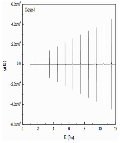
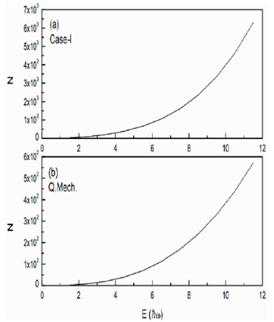
Figure 2 (a) Particle number N vs. E in units of ħω for Case I of isotropic oscillator. (b) Plot of Quantum results.
To obtain the splitting due to
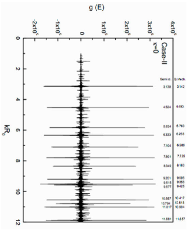
Figure 3 Total level density g(E) vs. kR0 for Case II of isotropic oscillator with κ = 0. The quantum results are also given for comparison.
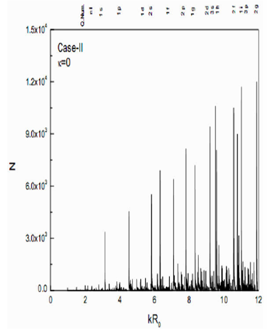
The particle numbers are calculated by using Eq. (41) and are shown in Fig. 4 as a function of kR 0 . Here, F F in terms of kR 0 is varied continuously from 1 to 12. Again the calculated N values are quite high as compared to quantum results, which can be reduced by including Pauli-principle in the trace formula. If we compare this plot with the quantum numbers which are also identified at the top of this plot, the following interesting features emerge:
The significant gaps in the kR 0 values are seen at the usual magic numbers of the spherical well, i.e., 2, 8, 20, 34, 58, 92 and 138.
The relative difference in peak heights referring to the quantum shells 1s, 1p 1d, 1f, 1g, 1h, and 1i is constant and is equal to 1 unit each. The relative increase of one unit in the peak height concerning its predecessor refers to the increase in angular momentum by one unit.
A sudden rise in the number peak among the nearest neighbors indicate the existence of a shell with a different quantum number ‘n’.
The repetition of a particular shell occurs in the spectrum at a particular value of kR 0 , if the relative ratio of the peak heights coincides with their respective ratio of kR 0 . For example, the ratio of peak heights of 2 and 1 is 2, which is the same as their ratios of kR 0 values. Hence from this analysis, the quantum number ‘n’ can be identified.
Another advantage of this study is to show the splitting of the eigenvalue spectrum by
including the
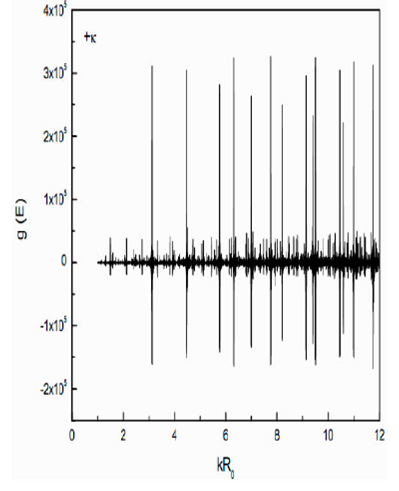
Figure 5.Total level density g(E) vs. kR0 for combination of Case II and positive sign with k in
In nuclear system with
Table I A comparison of eigenvalues, in terms of kR
0, of an isotropic oscillator of Case II, without and with
| n | l | Qmech. no. |
Scl. no. |
Scl. no.+ |
Scl. - |
| 1 | s | 3.142 | 3.138 | 3.124 | 3.151 |
| 1 | p | 4.493 | 4.524 | 4.483 | 4.566 |
| 1 | d | 5.763 | 5.834 | 5.762 | 5.906 |
| 2 | s | 6.283 | 6.333 | 6.320 | 6.345 |
| 1 | f | 6.988 | 7.104 | 6.999 | 7.209 |
| 2 | p | 7.725 | 7.801 | 7.762 | 7.841 |
| 1 | g | 8.183 | 8.349 | 8.210 | 8.489 |
| 2 | d | 9.095 | 9.201 | 9.134 | 9.268 |
| 3 | s | 9.356 | 9.515 | 9.403 | 9.520 |
| 1 | h | 9.425 | 9.577 | 9.502 | 9.753 |
| 2 | f | 10.417 | 10.557 | 10.461 | 9.753 |
| 1 | i | 10.513 | 10.794 | 10.582 | 11.007 |
| 3 | p | 10.904 | 11.017 | 10.978 | 11.056 |
| 2 | g | 11.657 | 11.881 | 11.754 | 12.008 |
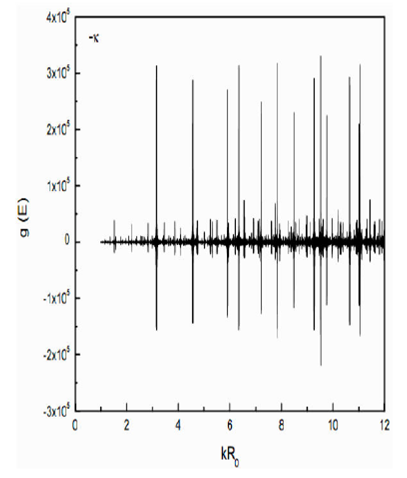
Finally, the total level density g(E) vs kR 0 , including both positive and negative signs with κ, is shown in Fig. 7, respectively, by solid and dotted curves. The resultant eigenvalue spectrum clearly shows the splitting.
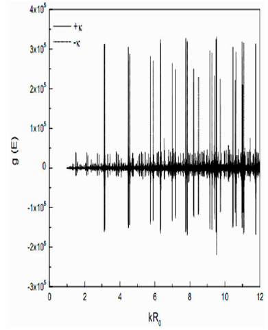
Figure 7 Total level density g(E) vs. kR0 for Case II including both positive and negative signs with κ in
The plot of the number of particles, vs kR 0 with both positive and negative signs of κ are shown by solid and dotted curves, respectively, in Fig. 8. It is evident from this plot that the dotted curve refers to the quantum mechanical case of j=l−(1/2), whereas the solid curves refer to j=l+(1/2). The number of particles shown by the dotted curve is less than those of a solid curve in a particular shell, which again supports the quantum mechanical observation. In order to get a reasonable separation in kR 0 at the magic numbers 28, 50, etc., we have to adjust the splitting parameter λ, which we have chosen equal to 0.2. Thus a complete semiclassical picture of the nuclear shell model is obtained, which will help predic the next magic numbers.
4.Conclusion
A trace formula for the level density of an isotropic harmonic oscillator with

