


 text new page (beta)
 English (pdf)
 Article in xml format
 Article references
 Send this article by e-mail
 Cited by SciELO
  Similars in
SciELO
Similars in
SciELO 
 Permalink
1. Introduction
Optical imaging of intrinsic signals (OIS) is a technique that employs a digital camera to record images of the brain, while specific wavelengths of light are shunned upon the cortical surface. Relative changes in reflected light intensity correspond to relative changes in the local concentrations of oxygenated hemoglobin and deoxygenated hemoglobin. OIS series of images represent a bidimensional functional map of hemodynamic signals, which are a proxy of neural activity [1]. Briefly, when a neuron fires, there is a localized consumption of oxygen revealed by an initial augmentation in deoxygenated hemoglobin. One or two seconds later, there is a large increase in cerebral blood flow and cerebral blood volume as a compensatory process to the initial oxygen consumption. This large discrepancy between oxygen utilization and supply prompts a delayed increase in the local concentration of oxygenated hemoglobin and the ensuing dilution of deoxygenated hemoglobin. Therefore, neural activity can be indirectly quantified and localized by measuring hemodynamic changes [2]. In small mammal models, OIs is usually performed through the intact skull of the animal, with the scalp carefully removed, as in this work. Certainly, with larger animals, OIS needs to carry out OIS through the thinned skull with a rotative tool [3]. Can be extended to study optogenetically evoked signals, although it requires transgenic mice expressing channelrhodopsin (ChR2) [4], it can be performed in isolated brain slices ex vivo [1] or facilitated through the use of an intracranial transparent window [5]. OIS has been employed as a diagnostic tool, taking advantage of the intrinsic contrast provided by hemoglobin, which allows imaging without the addition of external contrast reagents. Its numerous theoretical and empirical advantages position this modality as a strong candidate to study the brain in murine models of neurological conditions [6]. Two of the greatest advantages over other brain imaging modalities are the use of non-ionizing radiation and its moderate cost [5]. Conventional techniques used to acquire OIS images rely on scientific-grade charged-couple device (CCD) or complementary metal-oxide-semiconductor (CMOS) of the so-called scientific-grade, which cost between $2600 USD (PhotonFocus MV1-D1024E-160-CL-12) to $9000 USD (Tele-dyne DALSA Pantera 1M30), plus the added cost of a macro lens and a computer with a frame grabber. The use of a Raspberry Pi with its CMOS V2 camera module [7] retains the advantage of using nonionizing radiation and further reduces the cost by approximately 1.5 orders of magnitude. Hence, our motivation to explore this technique in a low-cost platform, which would empower the scientific community with a portable, inexpensive instrument to map the brain of small animal models. Functional imaging has been previously performed with a Raspberry and its camera [8], however extrinsic contrast, in the form of genetically modified mice expressing light-sensitive protein was employed. The use of wildtype mice provides a quick, simple, and inexpensive way to study brain function in a non-contact fashion with Raspberry-based OIS apparatus. The main goal of this work is to characterize the capabilities of this imaging setup free of extrinsic contrast and provide a proof of concept application in a mouse.
2. Methods
2.1. Optical setup and characterization
In our proposed low-cost imaging system, the Raspberry Pi 3 and its V2 camera module are used, as shown in Fig. 1b). This camera uses an 8 megapixel CMOS sensor (Sony IMX219) operating in the visible range, i.e from 400 to 700 nm. Video recording was set at 30 frames/second (fps) with a frame size of 256 χ 256 pixels, in raw-data format. This acquisition frequency avoids aliasing of physiological signals, such as cardiac frequency (~ 7 - 10 Hz) and respiration (~ 5 Hz). To achieve a field of view (FOV) of ~ 10 χ 10 mm, necessary to cover the convexity of the mouse cerebral cortex, the lens (focal length = 3.04 mm, f-number = 2.0) of the V2 module was unscrewed to the limit of its counterclockwise position, as described by Murphy et al. [8]. Images were acquired with diffuse illumination provided by either an (R) red (VCC VAOL-SR1XAX-SA) or a (G) green (VCC VAOL-ST1XAX-SA) high-power LED. At any single time, only one illumination source was used. LEDs were driven with a custom-made source based on a constant-current driver (XP power LDU2430S700-WD). The emission spectra of the LEDs were characterized by a portable spectrometer in the visible range, from 350 to 1000nm (Ocean Optics JAZ EL 350). These spectra are displayed alongside the absorption spectra of oxy- and deoxygenated hemoglobin [9] in Fig. 1a). Although the use of a single wavelength does not allow the obtention relative changes of deoxy- and oxy-hemoglobin, it reflects different components in cerebral tissue: total hemoglobin is the dominant signal with green illumination (λ = 535 nm), and deoxy-hemoglobin is the dominant component with red light (λ = 630 nm) [10].
Figure 1 a) Hemoglobin absorption spectra and LEDs emission spectra. b) Schematic layout of experimental montage, mouse head created with https://BioRender.com.
Dark frame assessment was performed per Pagnutti et al. [11]. In essence, ten dark frames were acquired at different electronic gain (ISO) values (seven levels between 100 and 800) with a fixed exposure time of 10 ms, and also at several exposure times, ranging from 1 ms to 33 ms in 1 ms increments, with ISO=100. Either the green or the red LEDs were used, along with a diffuser, as the light source of all the characterization experiments. Linearity characteristics of the V2 camera were determined as a function of ISO levels and as a function of exposure time. Camera linearity with ISO levels was assessed with an exposure time set to 10 ms ten bright-field images were captured for each ISO setting (seven levels from 100 up to 800). These bright-field images were temporally and spatially averaged to obtain a mean value. The linearity of the V2 camera with shutter speed, i.e. exposure time was carried out similarly as in the previous experiment, except that now ISO level was fixed at 100, and ten bright-field images were taken at shutter speeds from 1ms to 33 ms. These exposure times were chosen to allow recording at 30 frames per second. The coefficient of determination r2 was chosen as the metric of linearity. Sensor noise was characterized by analyzing 300 frames of data acquired at 10 ms exposure at ISO levels of 100, 200, 400, and 800, as described by Jacquot et al. [12]. Ten seconds of video, i.e. 300 frames were recorded at ISO levels of 100, 200, 400 and 800 at 10 ms exposure time. Different illumination levels were used to cover the dynamic range of the CMOS detector while avoiding saturation. The variance of these images was plotted against mean values. Negative USAF-1951 resolution target (R3L3S1N, Thorlabs, Newton NJ) was back-illuminated with diffuse light provided by either the green or the red LED. This allowed the estimation of resolution as the full width at half-maximum of the smallest discernable feature. Furthermore, the spatial frequency response was estimated according to the slanted-edge method, as described by the ISO 12233:2017 standard [13]. Using the same setup described a few lines above, a single image of an edge on the target, slightly slanted at ~ 28° off the vertical, was taken.
The spatial average of such a slanted edge gives the edge spread function (ESF), whose derivative is the Line Spread Function (LSF). When the Fourier transform on the spatial domain is applied to the LSF, the spatial frequency response of the system is obtained. This is called the modulation transfer function (MTF) and is defined as follows:
2.2. Animal preparation
In this proof-of-concept study one male C57BL/6 mouse was imaged (weight = 29 g, age = 23 weeks, Bioterio UASLP). All surgical procedures were approved by the local ethics committee and performed according to international recommendations. All mice were anesthetized intraperitoneally using urethane (U2500-100G Sigma-Aldrich) at a dose of 2 mg/g in a 10% (weight/volume) NaCl solution, taken from a freshly prepared stock solution (5 g urethane dissolved in 10 ml of 0.9% saline solution). Mice were installed in a custom head fixation setup and then scalp was carefully removed in order to expose the intact skull over the whole convexity of the cortex. Lidocaine (Xylocaine 5% gel) was topically applied to scalp incisions, as a local anesthetic. Mineral oil (NF-90 Golden Bell Reagents) was used to keep the skull moist and optically clear.
2.3. Functional connectivity
Optical measurements were considered at a single wavelength and normalized relative to the mean light intensity, as described by Eq. (2):
Data were band-pass filtered to the functional connectivity band (0.009-0.08 Hz), according to previous studies [6,14-16]. Images were spatially filtered with a 5x5 Gaussian kernel and then resampled from 30 fps to 1 fps. In order to minimize the influence of coherent variations common to all brain pixels, a global signal g was computed from the average of all those brain pixels and pixel-wise regressed from our measurements ∆I (t), yielding the regression coefficients ß g :
The removal of the global signal g from OIS data ∆I (t) generates the new image time series ∆I´ (t) which are now used for all further processing:
Global signal regression was performed with a general linear model (GLM) from the toolbox Statistical Parametrical Mapping [17]. Regions of interest (ROI) were placed on hemisphere-symmetric cortical areas, according to previous studies [15], as shown in Fig. 7a). Briefly, 6 ROIs in each hemisphere were selected from the frontal (F), cingulate (C), motor (M), somatosensorial (S), retrosplenial (R) and visual (V) brain regions. The coordinates for these ROIs were chosen based on the expected positions laid out by atlas-based parcellation techniques of previous works [14-16,18]. The time course of every ROI was computed from the average pixel value in each ROI, then a functional connectivity matrix was computed from the correlation between each pair of ROIs. Negative correlations were not considered for analysis owing to the difficulty in understanding their intricacies, such as the neural origin and interpretation of hemodynamic signals. All data processing here described was carried out under a MATLAB platform (The MathWorks, Natick, MA).
3. Results and discussion
In this work, a characterization of the Raspberry Pi V2 camera was performed. Dark noise was very low for low values of ISO (100, 200) and slightly larger for high ISO levels (320 - 800), as demonstrated by dark pixel distribution, depicted by Fig. 2a). Dark noise was mostly present around the corners of the sensor, and it is only noticeable with high ISO levels, as shown by panels B-E of Fig. 2.
Figure 2 Dark signal characterization: A) Distribution of pixel intensities over 10 frames per ISO level (seven values between 100 and 800). B) and C): mean value of R channel over 10 dark frames, for ISO=100 and ISO=800, respectively. D) and E): corresponding averages for G channel.
Raw data values were extremely linear with both ISO (Fig. 3a)) and shutter speed (Fig. 3b)). The coefficient of determination r 2 was very close to 1 for both green and red channels, albeit green channel linearity was higher regardless of exposure time.
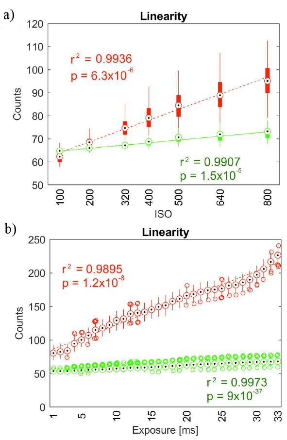
Figure 3 Linearity of camera response for both R and G channels: a) as a function of ISO levels and b) as a function of shutter speed (exposure time).
Sensor noise showed a positive linear scaling between variance σ2 and mean μ. The slope of this linearity increases with ISO levels for both channels, as shown by Fig. 4.

To assess the resolution of the system, a negative USAF-1951 resolution target was used as the testing device. This device consists of bars arranged as groups, and each group consists of six elements. Each element is made up of three vertical and three horizontal equidistant bars, and every element is associated with a corresponding resolution, based on the width of the bar. Under red light, the smallest resolvable feature was the third element of group 3, with 10.1 line pairs / mm or correspondingly a resolution of 99.2 μm, as depicted by Fig. 5a) and d). Using green illumination, we were able to clearly distinguish the fifth element in group 3, corresponding to a specification of 12.7 line pairs / mm or equivalently 78.7 μm. This is illustrated in Fig. 5c) and d).
Figure 5 PImaging system assessment using USAF 1951 resolution target with diffuse back-illumination of a) 𝜆 R = 630 nm and c) 𝜆 G = 535 nm. Intensity profile across the elements 1-6 of group 3, with 𝜆 R and 𝜆 G , were plotted in b) and d) respectively.
Figure 6a) shows the slanted edge images from which MTF values were computed. Panel B of the same figure displays the ESF. Resolving power determined by the 10-90 % ESF yielded 330 μm for the red band and 38.4 μm for the green channel. Using the derivative of the ESF, i.e. he LSF, shown in Fig. 6c), the resolution was determined as the full-width at half-maximum of the LSF. The measured FWHM for the red channel was 55.1 μm and for the green channel, 24.7 μm. The spatial frequency response of the system was assessed via the MTF, depicted in Fig. 6d). The limiting resolution was defined as the frequency response at 10% of MTF [19]. Red illumination yielded 24.1 cy/mm, while green light gave 52.3 cy/mm. As expected, a better resolution was obtained with shorter wavelengths.
Figure 6 Diagram of the slanted edge method to compute the spatial frequency response of the imaging system R and G channels: a) Edge target images, b) ESF estimated from image a,c) the resulting derivative of the ESF is the LSF and d) the Fourier transform of the LSF is the MTF.
Figure 7 textitIn vivo results a) Black circles denote the location of the seeds corresponding to functional cortices. Initials B and L are placed at bregma and lambda location respectively. Time traces for left and right visual seeds for b) red channel and c) green channel. Functional connectivity matrices for d) red channel (λ = 650 nm) and e) green channel (λ = 535 nm). ROIs notation: Frontal (F), cingulate (C), motor (M), somatosensorial (S), retrosplenial (R) and visual (V). The letter following an underscore denotes either left (L) or right (R) hemisphere.
Two contralateral cortical regions of the visual cortex were chosen to display functional connectivity analysis. Seed size and placement are indicated in the anatomical image taken under λ = 535 nm illumination, illustrated in Fig. 7a). Letters b and l describe bregma and lambda location, respectively. The corresponding time courses for each wavelength are shown in panels b and c of Fig. 7. Time traces of the visual cortex obtained under red light showed a correlation value r = 0.8069(p-value < 1 x 10-11 ) and those recorded under green light yielded a correlation value r = 0.8777(p ≃ 0). These results suggest that signals dominated by total hemoglobin (dominant in λ=535 nm) are more synchronized than those related to deoxy-hemoglobin (revealed by λ=650 nm). Connectivity matrices for each wave length are displayed in panels D and E of Fig. 7. It can be seen that images obtained under 535 nm light show increased connectivity this may be due to higher linearity and better spatial resolution of the green channel.
4. Conclusions
We demonstrated in vivo optical imaging of intrinsic signals of a mouse brain cortex using a cost-effective and compact system based on the Raspberry Pi 3 and its onboard V2 camera. We also provided a full characterization in terms of noise, linearity, and spatial resolution. In future work, group analysis will be done to provide robust measures of functional connectivity. The use of such a low-cost system in combination with an automated processing pipeline may facilitate the study of murine models with potential translation to clinical relevance in human brain diseases.

