


 text new page (beta)
 English (pdf)
 Article in xml format
 Article references
 Send this article by e-mail
 Cited by SciELO
  Similars in
SciELO
Similars in
SciELO 
 Permalink
1. Introduction
Perhaps the concordance or Λ-Cold Dark Matter (ΛCDM) model is the most successful via to reproduce the dynamics of our Universe [1] introducing the existence of dark entities known as dark matter (DM) and dark energy (DE). Despite its important achievements, the model suffers from different pathologies such as the flatness, the horizon problem (see [2] for an excellent discussion), the current Universe acceleration [3-5], among others. In particular, near or in the initial singularity and for times close to Planckian lengths and energies, it is necessary a quantum gravity theory (QG) to understand the universe in these regimes; in particular because gravity already plays a preponderant role at this quantum level. In this sense, the candidates to study this energy scale are for example string theory [6] or loop quantum gravity [7], being until now its predictions far from being falsifiable and its theoretical building far to be completely solved. These are some of the reasons of why the Wheeler-DeWitt (WDW) equation is still the cornerstone to address problems in QG scenarios and being also a great opportunity to pave the way in our search to find a final quantum gravity theoryi.
The noncommutativity in coordinates (NCC) were introduced in the late of 40’s [8], generating a great deal of interest in this area of research [9-13], impacting this boom in the study of the effects in the phase-space of the classical and quantum cosmology (QC) [14, 15]. It is noticeable to mention that the second case is a simplified approach to study the very early universe, where one could assume the effects of noncommutativity. As it is well known, in general, the configuration space in QC (superspace) is infinite-dimensional, but for the homogenous cosmologies (like our Universe), where the metric depends only on time, we can obtain a model with a finite degrees of freedom called the minisuperspace. In this context, like in noncommutative quantum mechanics [16-18], it is possible to introduce non-commutativity in a 2n-dimensional configuration space via the change of variables (Boop-shift) which are often referred to as the Seiberg-Witten map [13] and satisfy an extended Heisenberg algebra (see Appendix A). Therefore the traditional way to extract useful dynamical information and deal with the difficulties associated with solving the WDW equation in the challenging scenario of noncommutativity gravity is through the WKB-type method, and when it is used a (2 + 1)-minisuperspace model the wave function proposed takes the form shown in Appendix A; finding the associated Einstein-Hamilton-Jacobi (EHJ) equation, that is, a coupled system of two non-linear ordinary differential equations. To construct the EHJ equation and find analytical expressions, we observed the behavior, in a convenient limit, of functions involved addressing the analysis with a functions called asymptotic equals (see Appendix B), selecting the appropiate candidate of the respective equivalence class.
As a demonstration of the functionality of the method, we will apply it in the dynamical system derived from EHJ equation that comes from the FLRW metric, considering the non-commutativity in the space coordinates. In addition, together with the mentioned method, we associate in the noncommutative coordinate and momentum (NCCM)-KS cosmology a particular family of subsets, called Ultrafilter, that is relevant in some branches of mathematics, like topology where in many cases are used to construct examples and counter examples [24, 25], functional analysis and dynamical systems, when discrete systems are studied [26, 27]. The study of cosmology in some limits (asymptotic analysis) is well known and appears in problems related with the cosmological constant [19, 20], and the behavior of some models near to and far away from an initial singularity in certain kinds of cosmologies [21, 22] and in quintessence models [23]. Hence, the goal is support our work with the mathematical concepts mentioned and propose an analytical solution, unlike traditional methods studied in literature where is represented only in a integral form or solved numerically [28, 29]. Here we will take a step forward which will undoubtedly be useful for sketching the solution of the dynamical system associated to the EHJ equation from this approach.
This paper is organized as follows: In Sec. 2. we study the asymptotic behavior of functions in a semiclassical expression for the FLRW model with curvature k ≠ 0 and cosmological constant (Λ ≠ 0) in a NCC-frame. In Sec. 3. we obtain a semiclassical approach for the KS universe exploring a phase-space noncommutative extension and using again asymptotic analysis together with some properties of the collection of subsets introduced in the Appendix B, summarizing this procedure in Appendix C. By inspection, we compare our analytical expressions with the numerical solution of the dynamical system obtained from applying the semiclassical limit and our analysis in both models; also for the case of KS cosmology, with the numerical solution of the classical dynamical system. Finally, Sec. 4. deals with the conclusions and outlooks. We will henceforth use units in which c = ħ = 1.
2. Noncommutative FLRW Model
In order to use the asymptotic behavior, we first proceed to study the EHJ equation that comes from FLRW cosmology with the presence of the parameter θ. It is worth to notice that we will use FLRW model only as a laboratory to probe the effectiveness of the mathematical tool of asymptotically equal functions.
We start this study using the line element in this back-ground as:
where a(t) · e α(t) is the scale factor, N (t) is the lapse function and k is the curvature constant.
Based in previous work, Ref. [28], we calculate the canonical momenta for α and φ as
and the classical Hamiltonian for the case Λ ≠ 0 and k ≠ 0 reads
Thus, canonical quantization in the momenta and the Hamiltonian constraint for the ADM formulation, give us the WDW equation coupled to a scalar field and Λ in the form:
where 𝒩 = e 3α is chosen in order to fit the gauge. Since the effects of the deformation will reflect only in the WDW potential [30], when the noncommutativity in coordinates (x 1 = φ, x 2 = α) is applied in Eq. (4) and also the WKB-type method (Appendix A), we finally obtain the EHJ equation
Hence, we deduce the equations
with P
φ0
a positive decoupling constant and
Therefore applying (2) in (6a)-(6b) and choosing
The initial condition φ(t 0) = φ 0 give us φ(t) = φ 0−P φ0 (t− t 0). For Eq. (8b) defined in the interval (−∞,α 0) with α 0 < 0, under inspection, we have for the integrand
the following asymptotically equal function
with
where it is applied the initial condition
Proceeding in the same manner we obtain the commutative expressions for the general form as
In Table I we present, for decreasing values of t, the relative error that give the error rate (ER) between the numerical solution of the system (8a)-(8b) (with θ = 0 and θ ≠ 0) and the respective analytical expressions (13a) and (13b) for the commutative frame and (11) and (12) for the NCC one. Then Fig. 1 and Fig. 2 shows the plots for values of t in the interval [-1000, 0] observing that correspond to α’s in [-120, 0] and φ’s in [0, 400]. In Fig. 3 the factor that measures the evolutionii is analyzed, plotting this parameter with the analytical α and the numerical one in a commutative and NCC scenario, showing that when t is decreasing they are all similar. For a(t), when the values of t are near zero, the plots in both frames lies in the range [0, 1] (See the internal boxes in Fig. 3).
Table I Error rate between α’s, φ’s commutative and α’s, φ’s NCC (numerical and analytical expressions) with t 0 = 0, P φ0 = 2=5, θ = 5, Λ= k = 1 and the initial conditions α(t 0) = -2.30259 (commutative frame), α(t 0) = -4.77981 (NCC frame) and φ(t 0) = φ 0 = 10. See the text for more details.
| t | ER α conm ’s | ER φ conm ’s | ER α ncc ’s | ER φ ncc ’s |
|---|---|---|---|---|
| -100 | 2.33029% | 9.94 × 10 -14 % | 2.22202% | 6.9282% |
| -700 | 0.33% | 7.84 × 10 -14 % | 0.340638% | 1.19452% |
| -800 | 0.29207% | 6.89 × 10 -14 % | 0.298513% | 1.04973% |
| -900 | 0.259629% | 6.14 × 10 -14 % | 0.26566% | 0.936244% |
| -950 | 0.245969% | 5.83 × 10 -14 % | 0.251804% | 0.88823% |
| -990 | 0.236034% | 5.60 × 10 -14 % | 0.241718% | 0.853227% |
| -1000 | 0.233674% | 5.54 × 10 -14 % | 0.239321% | 0.844903% |
| -2000 | 0.11685% | 2.80 × 10 -14 % | 0.120175% | 0.427667% |
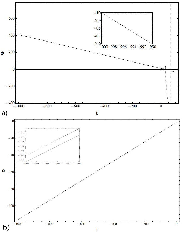
Figure 1 Plots for α, comparing in (a) the analytical expression (13b) (dashed line) and numerical solution of Eqs. (8a) and (8b) with θ = 0 (pointed line) and in (b) the analytical expression obtained in Eq. (11) (dashed line) with the solution of Eqs. (8a) and (8b) in a NCC frame (θ = 5), both under t 0 = 0, P φ0 = 2=5, Λ = k = 1 and the initial conditions α(t 0) = -2.30259 and α(t 0) = -4.77981, respectively.
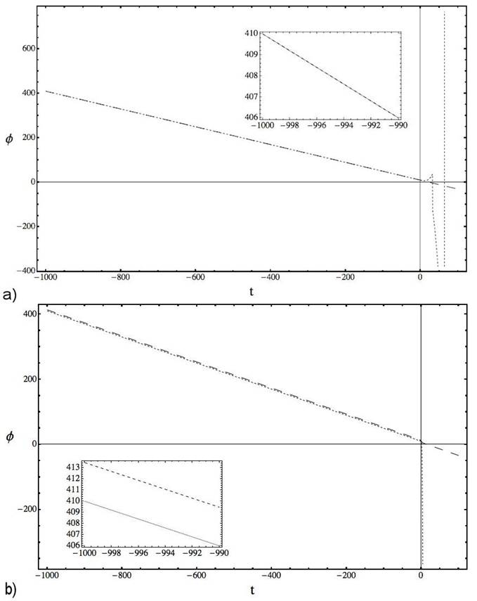
Figure 2 Plots for φ, comparing in (a) the analytical expression (13a) (dashed line) and numerical solution of Eqs. (8a) and (8b) with θ = 0 (pointed line) and in (b) the analytical expression obtained in Eq. (12) (dashed line) with the solution of Eqs. (8a) and (8b) in a NCC scenario (θ = 5) both under the same conditions that Fig. 1. The initial condition is φ(t 0) = φ0 = 10.
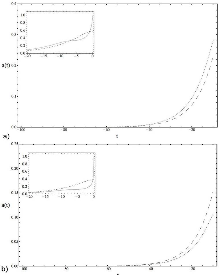
Figure 3 Plots of the scale factor exp(α) in a commutative (a) and a NCC (b) frame using the numerical solution of Eqs. (8a), (8b) (pointed line) and the expressions (8a), (11) (dashed line). For the commutative frame we make θ = 0 in the system and the same conditions that in Fig. 1 are considered.
3. Noncommutative KS Universe
In this section we are not only going to apply an asymptotic treatment, also we will introduce the conceptsiii shown in Appendix B looking for analytical expressions for the associated dynamical system that comes for the noncommutative space-space and momentum-momentum variables of the EHJ equation in the KS universe.
We start with the line element in the Misner parametrization [31]:
where X and Y are the scale factors. Following the same recipe as in Sec. 2, the WDW equation [15] is:
As the authors of Ref. [28] find, the momenta are
and remembering Appendix A, with the presence of the parameters θ and η (x 1 = β, x 2 = Ω), give the equation
where R(Ω) is defined as:
being σ as in the first Appendix.
In addition, noticing that
hence using the last approximation in (17) can be derived the system of equations:
where P β0 is like in Sec. 2 and E θ is a constant with the property
With the relations (16) and taking
The solution of Eq. (22a) with β(t 0) = β 0, give us
and for the parameter t it is possible to express in quadratures as
In the case where η → 0, Eqs. (23) and (24) are reported in literature (see [28] for details). To extract an analytical representation for the minisuperspace variables, in Appendix C we suggest a mathematical procedure to obtain an asymptotically equal function for G θ,η . Therefore, using (B.2) and (C.6), we find the expression
considering Ω(t 0) = Ω0 give C = (ln(Ω0) + ηt 0)η -1 and
The behavior of the above expressions versus the numerical solution of the system (22a)-(22b) for t ∈ [-1000, -100] (or values of Ω in the interval [22026.5, 1037]) are in Fig. 4, where similarities for small t’s are notorious. For example, taking t = -1000, -990, -950, -900. - 800, we have for Ω that the quotient between the numerical solution and the analytical expression is 1.00038 corresponding to a relative error (or ER) of 0.037%. Making the same for β we get that the quotients are 0.94444 and the error rate produced is 5.8824%. From the above we can consider that the numerical solution and Ω A are asymptotically equivalent when t → -∞, finding a similar behavior for β A .
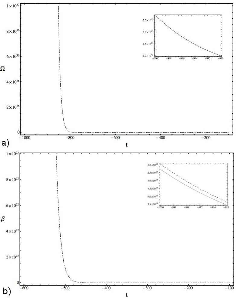
Figure 4 Plots of Ω A and β A (dashed line) comparing with numerical solutions of (22a), (22b) (pointed line), where t 0 = -100, P β0 = 2/5, θ = 5, η = 0.1, C = 1.5 × 10 -5 also considering the initial conditions Ω(t 0) = Ω0 = 2.20265 × 10⁴ and β(t 0) = β 0 = 4.68142 × 10⁴.
Now, the noncommutative relations imposing between the coordinates and their momenta in the modified Poisson algebra are:
giving the classical equations of motion:
An analytical solution of this system is beyond reach given and the distributions of the variables involved; hence, in Fig. 6 and 7 we present the numerical solutions Ω
N
, β
N
for Eqs. (28a)-(28d). Let
for t ∈ I
n
= [
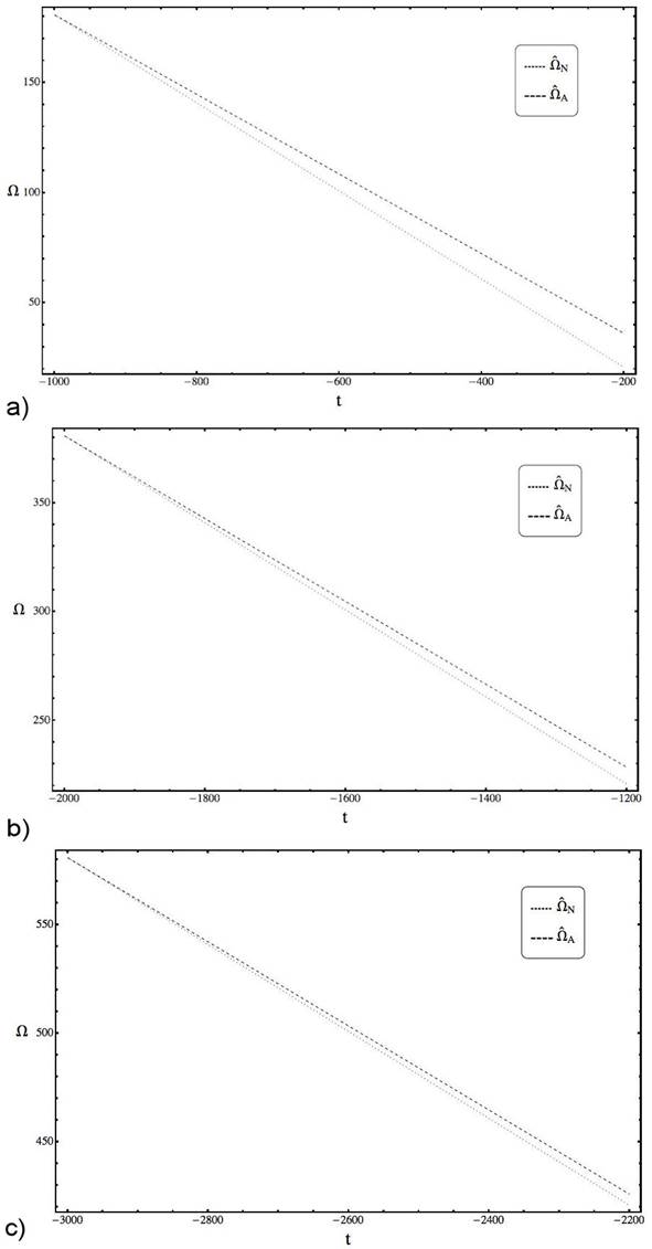
Figure 5 Plots of
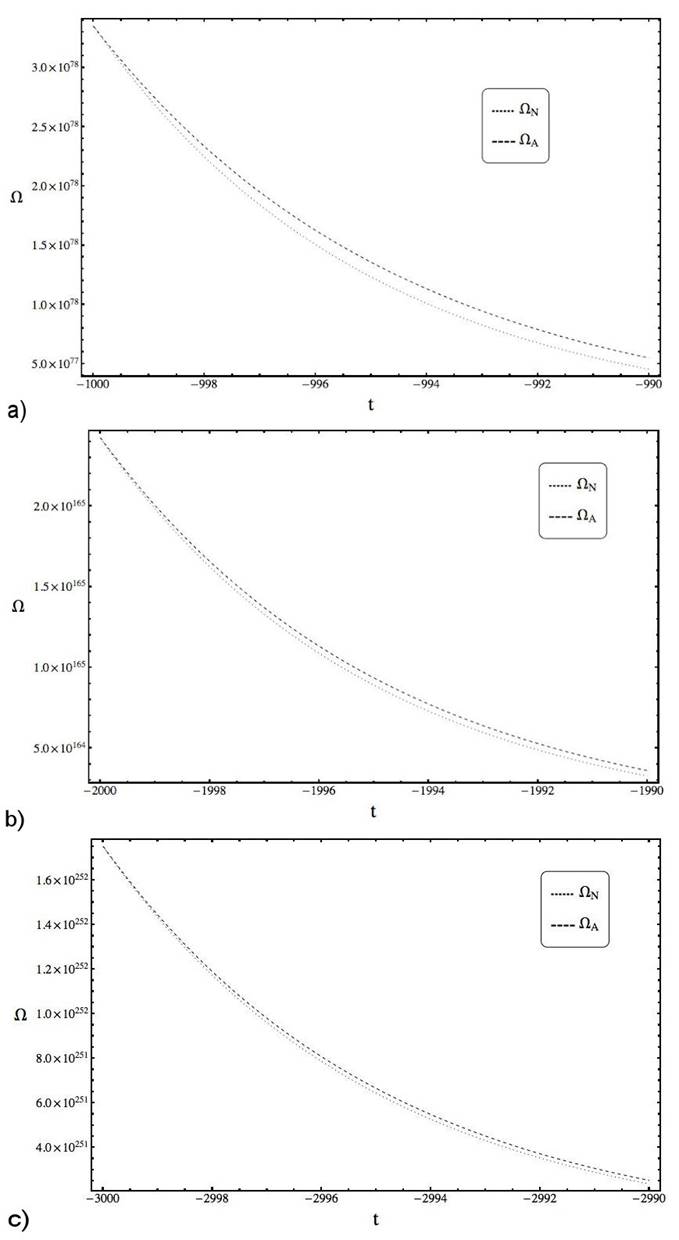
Figure 6 Plots of Ω N (dotted line) and Ω A (dashed line) in the intervals [-1000, -200] with q n,t = 1.80811, [-2000, -1200] with q n,t = 1.90406 and [-3000, -2200] with q n,t = 1.93604, where t 0 = -100, θ = 5, η = 0.1, C = 1.5 × 10 -5 also considering the initial conditions Ω(t 0) = Ω0 = 2.20265 × 10⁴ and β(t 0) = β 0 = 4.68142 × 10⁴, P Ω(t 0) = 0, P β (t 0) = 2=5.
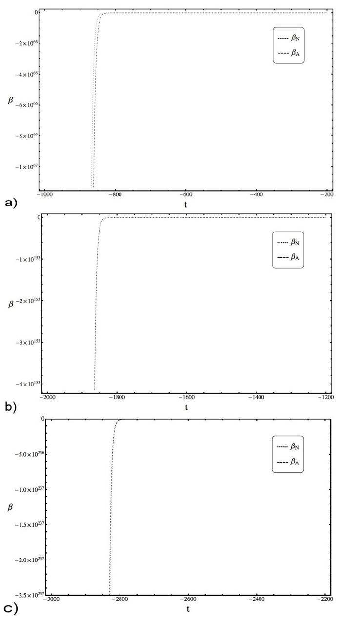
Figure 7 Plots of Ω N (dotted line) and Ω A (dashed line) in the intervals [-1000, -200] with q n,t = 1.80811, [-2000, -1200] with q n,t = 1.90406 and [-3000, -2200] with q n,t = 1.93604, where t 0 = -100, θ = 5, η = 0.1, C = 1.5 × 10 -5 also considering the initial conditions Ω(t 0) = Ω0 = 2.20265 × 10⁴ and β(t 0) = β 0 = 4.68142 × 10⁴, P Ω(t 0) = 0, P β (t 0) = 2=5.
and t n = t. The sequence {α i,ti } is divergent but have a notorious property. if {∣Z i ∣} is the sequence of cardinalities of the sets Z i of consecutive zeros (or the significative number is the same), we note that it also diverges since the number of consecutive zeros increases as t decreasesv and it is possible to treat q n,t as a constant when t → -∞vi, then under these assumptions we have
In Table II we check the error rate (ER) between
Tabla II. Error rate between
| t | n | q n,t | ER Ω’s |
|---|---|---|---|
| -200 | 1 | 1.80811 | 73.7653% |
| -225 | 1 | 1.80811 | 57.6173% |
| -1000 | 32 | 1.80811 | 0.0000389% |
| -1025 | 33 | 1.90406 | 5.03481% |
| -1200 | 40 | 1.90406 | 3.4769% |
| -2000 | 72 | 1.90406 | 0.00038% |
| -2025 | 73 | 1.93604 | 1.61664% |
| -2200 | 80 | 1.93604 | 1.2169% |
| -3000 | 112 | 1.93603 | 0.0001836% |
| -3025 | 113 | 1.95203 | 0.798575% |
| -3200 | 120 | 1.95203 | 0.618331% |
| -4000 | 152 | 1.95203 | 0.0001362% |
| -5000 | 192 | 1.95203 | 0.488977% |
| -6000 | 232 | 1.95203 | 0.812403% |
Finally, in Fig. 6 and 7 we present plots of Ω N , Ω A and β N , -β A showing the similarities with the numerical solutions
4. Conclusions and Outlooks
In this paper we have presented noncommutative quantum cosmology through the help of the WKB-type method for the WDW equation. Here, the homogeneous cosmologies in a NCC and NCCM frame are investigated. Although in both models the behavior of the functions (see the integrands in (8b) and (24) in the respective limit) are similar, we observe that there are many possibilities for an asymptotic function (see Appendix C) and the selection of the function in the equivalence class vary, being more natural for the FLRW model. The element chosen in the KS metric is relevant in the analysis, since it generates the associated ultrafilter and is not always possible to know it in an explicit way, given the maximality of this family.
In the FLRW model, when θ → 0 in α and φ, we obtain the commutative expressions for the general form and if k = 0 in Eqs. (11) and (12) we have the commutative and NCC solutions in the case k = 0, Λ ≠ 0 reported previously in literature (see Ref. [28]). In addition, making Λ = 0 together with
In the KS universe this significance is reflected when the classical system is considered, since in previous works the noncommutativity extension of this model is studied [29,32-34], extending our analysis and using the analytical form for Ω we get proposals that fits, in the limit imposed, with the numerical solution of the classical system. In the expression for Ω we take care to preserve the asymptotical behavior that is reflected in the refinement of the values q n,t , but remembering that when t → −∞ (large Ω) this value can have a constant treatment. Here, it is important to bear in mind that the presence of the parameter of noncommutativity in momenta could be of relevance for the selection of possible initial states in the early Universe [29]. The Equation (30) is a divergent sum and we use only one significative number to estimate the quotient, this leave the chance to study another expression for r n . For example, the equation:
where a 0 is treated like a constant number in the region R (remember that the sets Z i become to get bigger as t decrease), t i ∈ I i ⊂ R and{s i,ti }is a convenient increasing sequence.
When we deal with asymptotic equivalent functions, we have to consider that their relative error is zero as Tables I, II and Figs. 6, 7 show. Indeed, in the comparison between the analytic proposals versus the numerical solutions, the error remains sufficiently small to be able to consider them as a good approximation (the analytical expression and numerical solution can be treated like asymptotically equal). Indeed, we notice that on a complete deformed space it is possible to obtain an expression for the FLRW model, proceeding similarly as in the KS universe.
Since it have been shown an unexpected connection of some set of theoretical concepts with quantum mechanics as well as with cosmology [35,36], the treatment in this scenario via this ideas is the following steps to explore, taking the formal models in ZFC (Zermelo-Fraenkel-Axiom of Choice) and hence forcing that special tool to make the shift from the micro to macro scale. Finally, others scenarios in quantum cosmology can be analyzed in order to explore the feasibility of the mathematical methods presented in this paper; however this is work that will be done elsewhere.

