1. Introduction

Blazars are a subclass of Active Galactic Nuclei (AGN) and the dominant extra galactic population in gamma-rays ^[1]. These objects show rapid variability in the entire electromagnetic spectrum and have non thermal spectra which implies that the observed photons originate within the highly relativistic jets oriented very close to the observers line of sight ^[2]. Due to the small viewing angle of the jet, it is possible to observe the strong relativistic effects, such as the boosting of the emitted power and a shortening of the characteristic time scales, as short as minutes ^[3,4]. Thus, these objects are important to study the energy extraction mechanisms from the central super-massive black hole, physical properties of the astrophysical jets, acceleration mechanisms of the charged particles in the jet and production of ultra high energy cosmic rays, very high energy γ-rays and neutrinos.

The spectral energy distribution (SED) of these blazars has a double peak structure in the v - vF_v plane. The low energy peak corresponds to the synchrotron radiation from a population of relativistic electrons in the jet and the high energy peak believed to be due to the synchrotron self Compton (SSC) scattering of the high energy electrons with their self-produced synchrotron photons ^[5,6]. Depending mostly on the optical spectra, blazars can be divied into BL Lacertae objects (BL Lacs) and flat- spectrum radio quasars (FSRQ) [⁷]. Based on the location of the first peak, BL Lacs can be further classified into low energy peaked blazars (LBLs) (νsynpeak < 10¹⁴Hz), intermediate energy peaked blazars (IBLs) (10¹⁴Hz < νsynpeak < 10¹⁵ Hz) and high energy peaked blazars (HBLs) (νsynpeak >10¹⁵Hz). As leptons (e ^±) are responsible for the production of the SED, this is called the leptonic model and in general is very successful to explain the multiwavelength emission from blazars and Fanaroff-Riley Class I galaxies (FR-I) ^[9-12]. The inevitable outcome of the leptonic models is that flaring at TeV energy should be accompanied by a simultaneous flaring in the synchrotron peak. However, non observation/suppression of low energy counterparts have been observed in many flaring blazars, for example, flare of May 2002 from the HBL 1ES 1959+650 ^[13-15] and 2004 flare from Markarian 421 ^[16]. These observations are in favor of hadronic model and/or hybrid (hadronic + leptonic) models. It is to be noted that, recent observation of the high energy neutrino event by IceCube neutrino observatory is correlated with a flaring blazar ^[17,18]. So very high energy (VHE) protons/nuclei should be produced by the blazar so that their interaction with the surrounding background can produce pions and subsequent decay of pions will produce neutrinos and gamma-rays. This shows that hadronic models play important role here.

Flaring seems to be the major activity of the blazars which is unpredictable and switches between quiescent and active states involving different time scales and fluxes. While in some blazars a strong temporal correlation between X-ray and multi-TeV γ-ray has been observed, outbursts in some other have no low energy counterparts (orphan flaring) ^[15,16] and explanation of such extreme activity needs to be addressed through different mechanisms. It is also very important to have simultaneous multiwavelength observations of the flaring period to constrain different theoretical models of emission in different energy regimes.

Different theoretical models have been proposed to explain the flaring from AGN and its subclasses. These models are mainly clssified into two categories: the leptonic models and the hadronic models. In the leptonic model scenario, the high energy electrons upscatter the low energy photons in the jet through the SSC process and the photons can be in the GeV-TeV region. This model has severe limitations to explain VHE γ-rays and the orphan flaring observed in many blazars. The multi-zone leptonic model can explain these high energy emissions, however, one has to increase the number of parameters in the model. In the hadronic synchrotron-proton blazar model ^[19,21], emission of synchrotron photons from protons take place. In this scenario, the Fermi accelerated protons in the jet magnetic field, emit synchrotron radiation which will be suppressed by a factor of m^-4_p, where m_p is the proton mass. So ultra high energy proton flux is needed to explain the VHE gamma-rays. It also needs a strong magnetic field for the synchrotron process to be effective, but a strong magnetic field in the jet is not very usual. In the jet-in-jet model of Giannios et al. ^[22] minijets are formed within the jet due to flow instabilities and these minijets move relativistically with respect to the main jet flow. The interaction of the daughter jets with the main jet are responsible for the production of VHE gamma rays. While the minijets are aligned with our line of sight, the VHE gamma rays are beamed with large Doppler factor. This scenario can explain the 2010 flare of the radio galaxy M87 but does not provide a quantitive prediction of the light curve of the flare. The lepto-hadronic model ^[23] fits to the low energy γ-ray spectrum by Large Area Telescope (LAT) and High-Energy Stereoscopic System (H.E.S.S.) low state but not the flaring state. Similarly, the magnetosphere model ^[24-26] can explain the hard TeV spectrum but in this case also there is no detailed quantitive predication for the VHE light curve. Also interaction of Fermi acclerated protons with the MeV photons emitted by the Wein fireball in the base of the jet can explain the orphan falring from 1ES 1959+650 and Mrk 421 ^[27]. It is well known that EBL plays an inportant role for the attenuation of γ-rays even from the nearby blazars and this model does not take into account the EBL effect. The VHE SED of blazars are modelled using different hadronic models ^[28-31]. Using the hadronic models, the high energy cosmic ray and the neutrino fluxes are also estimated.

In a series of papers Sahu et al. ^[35-42] have explained the GeV-TeV flaring from many blazars using photohadronic scenario. In this scenario, Fermi accelerated protons interact with the background photons in the jet environment to produce Δ-resonance. Subsequent decay of the Δ-resonance to pions can produce VHE photons and neutrinos. The produced gamma-rays can explain very well the observed spectra from the flaring blazars.

The TeV photons of the flare can interact with the background soft photons in the jet to produce e⁺e^- pairs. However, production of the lepton pair within the jet depends on the size of the emitting region and the photon density in it. Also the required target soft photon threshold energy ∈_γ ≥ 2m²_e/E_γ is needed. It has been observed that the jet medium is transparent to pair production where the optical depth is very small ^[35,43]. Also the TeV photons on their way to Earth can interact with the extragalactic background light (EBL) to produce the lepton pair. TeV photons from the sources in the cosmologically local Universe (low redshift sources) are believed to propagate unimpeded by the EBL, although the effect is found to be non negligible ^[43].

In this work the goal is to use the photohadronic model of Sahu et al. ^[35] and different template EBL models ^[47,48] to explain the observed GeV-TeV flares from different HBLs. In this article, I review the photohadronic model of Sahu et al. and discuss about its applicability to explain the flaring events from high energy blazars. The plan of the papers is as follows. In Sec. 2 a short account of different EBL models is given. In Sec. 3 a detail discussion about the photohadronic model and the kinematical condition for the process ργ → Δ and its subsequent decay is given. Also the relation between the observed GeV-TeV gamma-ray flux and the gamma-ray from the photohadronic process is shown. Sec. 4 is dedicated to discuss the results of different flaring blazars and compare the results with other models. In Sec. 5 a general remark is given regarding the problems of different models. Finally I summarize the photohadronic model and discuss about the future research in this field in Sec. 6.

2. EBL Models

A distinctive feature of the high energy γ-ray astronomy is that the high energy gamma-rays undergo energy dependent attenuation en route to Earth by the intervening EBL through electron-positron pair production ^[44]. This interaction process not only attenuates the absolute flux but also significantly changes the spectral shape of the VHE photons. The diffuse EBL contains a record of the star formation history of the Universe. A proper understanding of the EBL SED is very important for the correct interpretation of the deabsorbed VHE spectrum from the source. The direct measurement of the EBL is very difficult with high uncertainties mainly due to the contribution of zodiacal light ^[45,49], and galaxy counts result in a lower limit since the number of unresolved sources (faint galaxies) is unknown ^[50].

Keeping in mind the observational constraints and the uncertainty associated with the direct detection of the EBL contribution, several approaches with different degrees of complexity have been developed to calculate the EBL density as a function of energy for different redshifts. A wide range of models have been developed to model the EBL SED based on our knowledge of galaxy and star formation rate and at the same time incorporating the observational inputs ^{[46-48,51-54]}. Mainly three types of EBL models exist: backward and forward evolution models and semi-analytical galaxy formation models with a combination of information about galaxy evolution and observed properties of galaxy spectra. In the backward evolution scenarios ^[52], one starts from the observed properties of galaxies in the local universe and evolve them from cosmological initial conditions or extrapolating backward in time using parametric models of the evolution of galaxies. This extrapolation induces uncertainties in the properties of the EBL which increases at high redshifts. However, the forward evolution models ^[47,51] predict the temporal evolution of galaxies forward in time starting from the cosmological initial conditions. Although, these models are successful in reproducing the general characteristics of the observed EBL, cannot account for the detailed evolution of important quantities such as the metallicity and dust content, which can significantly affect the shape of the EBL. Finally, semi-analytical models have been developed which follow the formation of large scale structures driven by cold dark matter in the universe by using the cosmological parameters from observations. This method also accounts for the merging of the dark matter halos and the emergence of galaxies which form as baryonic matter falls into the potential wells of these halos. Such models are successful in reproducing observed properties of galaxies from local universe up to z∼6.

3. Photohadronic Scenario

In general, in the leptonic one-zone synchrotron and SSC jet model the emitting region is a blob with comoving radius R'_b (where ' implies the jet comoving frame and without prime are in the observer frame), moving with a velocity β_c corresponding to a bulk Lorentz factor Γ and seen at an angle θ_ob by an observer which results with a Doppler factor D = Γ^-1 (1 - β_c cosθ _ob )-1 ^[10,15]. The emitting region is filled with an isotropic electron population and a randomly oriented magnetic field B’. The electrons have a power-law spectrum. The energy spectrum of the Fermi-accelerated protons in the blazar jet is also assumed to be of power-law. Due to high radiative losses, electron acceleration is limited. On the other hand, protons and heavy nuclei can reach Ultra-High Energy (UHE) through the same acceleration mechanism.

The photohadronic model discussed here relies on the above standard interpretation of the leptonic model to explain both low and high energy peaks by synchrotron and SSC photons respectively as in the case of any other AGN. Thereafter, it is assumed that the flaring occurs within a compact and confined volume of size R'_f inside the blob of radius R'_b. The geometrical description of the jet structure during a flare is shown in Fig. 1. In this scenario the internal and the external jets are moving with almost the same bulk Lorentz factor Γin ≃ Γext ≃Γ and the Doppler factor D as the blob (for blazars Γ≃D). Within the confined volume, the injected spectrum of the Fermi accelerated charged particles have a power-law, and for the protons with energy E_p it is given as

where the spectral index α ≤ 2 [⁵]. Also in this small volume, the comoving photon number density n'_γ,f (flaring) is much higher than rest of the blob n'_γ (non-flaring).

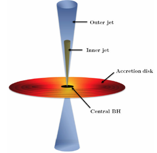
Figure 1 Geometry of the flaring of HBL: the interior compact cone (jet) is responsible for the flaring event and the exterior cone corresponds to the normal jet. 

The dominant mechanism through which the high energy protons interact with the background photons in the inner jet region is given by

which has a cross section σ_Δ ∼ 5 x 10^-28 cm². Subsequently, the charged and neutral pions will decay through π+→e+νeνμν¯μ and π⁰ → γγ respectively. The inner compact region has a photon density much higher than the outer region. Due to the adiabatic expansion of the inner jet, the photon density will decrease when it crosses into the outer region. We assume the scaling behavior of the photon densities in the inner and the outer regions. Mathematically we can express this as

i.e. the ratio of photon densities at two different background energies ∈_γ1 and ∈_γ2 in the flaring (n'_γ,f) and in the non-flaring (n'_γ) states remains almost the same. The photon density in the outer region is known to us from the observed flux. So by using the above relation, we can express the unknown inner photon density in terms of the known outer density which can be calculated from the observed flux in the usual way using the observed/fitted spectral energy distribution (SED). Henceforth, for our calculation, we shall use n’_γ and its corresponding flux rather than the one from the inner jet region which is not known.

4. Results

From the continuous monitoring and dedicated multi-wavelength observations of the nearest HBLs Markarian 421 (Mrk 421, z=0.0308), Mrk 501 (z=0.033 [^58,59]) and 1ES 1959+650 (z=0.047 ^[60]), several major multi-TeV flares have been observed ^[61-65]. Strong temporal correlation in different wavebands, particularly in X-rays and VHE γ-rays has been observed in some flaring events. However, in some other flaring events no such correlation is observed [^15,16], which seems unusual for a leptonic origin ^[9,10,12,66] of the multi-TeV emissions and needs to be addressed through other alternative mechanisms ^{[55,67-71,98]}. Below we shall discuss the flaring of Mrk 421, Mrk 501 and 1ES1959+650 separately.

4.1 Markarian 421

Mrk 421 was the first extragalactic source detected in the multi-TeV domain ^[72] and also it is one of the fastest varying γ-ray sources. It has a luminosity distance d _L of about 129.8 Mpc and its central supermassive black hole is assumed to have a mass M_BH ≃ (2-9)x10⁸ M_ʘ corresponding to a Schwarzschild radius of (0.6-2.7) x 10¹⁴ cm and the Eddington luminosity L_Edd = (2.5 - 11.3) x 10⁴⁶ erg s^-1. The synchrotron peak (1st peak) of its SED is in the soft to medium X-ray range and the SSC peak (2nd peak) is in the GeV range. Through dedicated multi wavelength observations, the source has been studied intensively. These studies show a correlation between X-rays and VHE γ-rays. A one-zone SSC model explains the observed SED reasonably well ^[73]. Several large flares were observed in 2000 - 2001 ^[74-76] and 2003 - 2004 ^[16,77]. During April 2004, a large flare took place both in the X-rays and the TeV energy bands. The flare lasted for more than two weeks (from Modified Julian Date (MJD) 53,104 to roughly MJD 53,120). Due to a large data gap between MJD 53,093 and 53,104, it is difficult to exactly quantify the duration. The source was observed simultaneously at TeV energies with the Whipple 10 m telescope and at X-ray energies with the Rossi X-ray Timing Explorer (RXTE) ^[16]. It was also observed simultaneously at lower wavelengths (both radio and optical). During the flaring it was observed that, the TeV flares had no coincident counterparts at longer wavelengths. Also it was observed that the X-ray flux reached its peak 1.5 days before the TeV flux did during this outburst. Remarkable similarities between the orphan TeV flare in 1ES 1959+650 and Mrk 421 were observed, including similar variation patterns in the X-ray spectrum. A strong outburst in multi-TeV energy in Mrk 421 was first detected by Very Energetic Radiation Imaging Telescope Array System (VERITAS) observatory on 16th of February 2010 and follow up observations were done by the HESS telescopes during four subsequent nights ^[61].

A six month long multi-instrument campaign by the Major Atmospheric Gamma Imaging Cherenkov Telescopes (MAGIC) telescopes observed VHE flaring from Mrk 421 on 25th of April 2014 and the flux (above 300 GeV) was about 16 times brighter than the usual one. This triggered a joint ToO program by X-ray Multi-mirror Mission - Newton (XMM-Newton), VERITAS, and MAGIC instruments. These three instruments individually observed approximately 3 h each day on April 29, May 1, and May 3 of 2014 ^[78]. The simultaneous VERITAS-XMM-Newton observation is published recently and it is shown that the observed multiwavelength spectra are consistent with one-zone synchrotron self-Compton model ^[78].

The observed multi-TeV flux from the above flaring events are EBL corrected and for this correction well known EBL models of Dominguez et al. ^[46] (EBL-D) and Inoue et al. ^[48] (EBL-I) are used. In Fig. 1 the attenuation factor for these two models as functions of observed gamma-ray energy E _γ are shown and both are practically the same in all the energy ranges (there is a minor difference in the energy range 600 Gev ≤ E _γ ≤ 1TeV.

4.1.1 The flare of April 2004

The multi-TeV flare of April 2004 was the first flare observed in multiwavelength by the Whipple telescope in the energy range 0.25TeV(6.0 x 10²⁵ Hz) ≤ Eγ ≤ 16.85TeV(4.1 x 10²⁷ Hz) and it was difficult to explain by one-zone leptonic model [¹⁶]. As discussed above, the photohadronic interpretation of the flare data needs the leptonic model as input and here the one-zone leptonic model of Ref. ^[16] (lep-1) is used. In this model the bulk Lorentz is Γ = D = 14. The above range of E_γ corresponds to the Fermi accelerated proton energy in the range 2.5 TeV ≤ E_p ≤ E_p ≤ 168 TeV and the corresponding background photon energy is in the range 23.6MeV(5.7 x 10²¹Hz) ≥ ϵ_γ ≥ 0.35MeV(8.4 x 10¹⁹Hz). This range of ∈_γ is in the low energy tail region of the SSC SED and its flux is expressed as power-law given in Eq. (24) with Φ₀ = 6.0 x 10^-10 erg cm^-2s^-1 and β = 0.48 which is shown in Fig. 2.

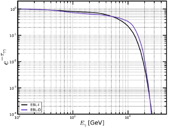
Figure 2 At a redshift of z = 0:031, the attenuation factor as a function of E _γ for different EBL models are shown for comparison. 

Very good fit to the multi-TeV flare data is obtained for α = 2.7, and the normalization constant A _γ for EBL-D is 2.3 and for EBL-I is 2.5 respectively which are shown in Fig. 3. Below 4 TeV both these EBL models fit the data very well, above this energy there is a slight difference due to the change in the attenuation factor. It is observed that EBL-D fits better than the EBL-I. To compare the photohadronic model fit without EBL correction but with an exponential cut-off (dN/dE_γ α E^-α_γ exp (-E_γ / E_c)) [³⁸], and the multi-zone leptonic model fit (magenta curve) [¹⁶] are also shown in the same figure (red curve). It can be seen from Fig. 3 that the multi-zone fit is not so good compared to other fits for E_γ ≤ 15 TeV. However, for higher energy it has the same behavior as EBL-D and EBL-I. With the exponential cut-off scenario, a good fit is obtained for the spectral index α = 2.7 and the cut-off energy E_C = 6.2 TeV. Again comparing this with the EBL corrected models, below 4 TeV, all these fits are exactly the same. However, above 4 TeV we observe some discrepancy among these fits and above 10 TeV the fits of EBL-D and EBL-I fall faster than the exponential cut-off scenario. Comparison of EBL-I with the exponential cut-off scenario shows that, for E_γ ≤ 10 TeV both e^-Eγ/Ec and e^-τγγ are almost the same and above 10 TeV the attenuation factor falls faster than the exponential cut-off. The intrinsic flux in EBL-D and EBL-I are almost the same and having power-law behavior with Fγ,in∝Eγ-0.18. Even though all these models fit quite well to the observed data below 20 TeV energy range, the deviation is appreciable above 20 TeV between the EBL corrected plots and the exponential cut-off. So observation of VHE flux above ∼ 30 TeV will be a good test to constrain the EBL effect on the VHE gamma-rays from Mrk 421.

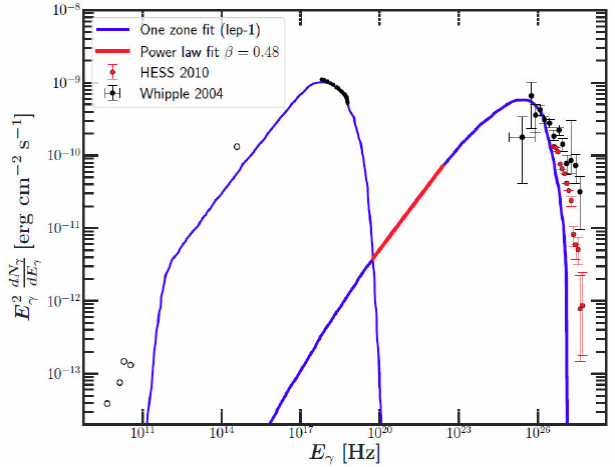
Figure 3 The fit to the tail region of the SSC SED (lep-1) [16] with the power-law as given in Eq. (24) with Φ₀ = 6:0 x 10^-10 erg cm^-2 s^-1 and β = 0:48 (red curve). 

By comparing different time scales i.e. expansion time scale, interaction time scale of ργ interaction and using the fact that the high energy proton luminosity to be smaller than the Eddington luminosity in the inner jet region of size R'_f ≃ 3x10¹⁵ m, the range of optical depth for the Δ-resonance production is estimated as 0.02 < π_ργ < 0.13. This corresponds to a photon density in the inner jet region as 1.3×1010 cm-3<n'γ,f<8.9×1010cm-3. The TeV photons produced from the neutral pion decay will mostly encounter the SSC photons in the energy range 0.35 MeV ≤ E_γ ≤ 23.6 MeV. The pair production cross section for ∈_γ ≥ 0.35 MeV is very small (σ_γγ ≤ 10^-30 cm^-2) which corresponds to a mean free path of λ_γγ ≥ 10¹⁹ cm for the multi-TeV gamma-rays, larger than the outer jet size. So, the TeV photons will not be attenuated much due to the e⁺e^- pair production.

4.1.2 The flare of February 2010

On 16th of February 2010, a strong outburst in multi-TeV gamma-rays from Mrk 421 was observed by VERITAS telescopes and follow up observations were carried out by HESS telescopes from 17th to 20th of February a total of 6.5 h. These data were taken in 11 runs with each run ∼ 28 minutes duration [⁶¹]. The HESS telescopes observed the flare in the energy range 1.67 TeV (4.0 x 10²⁶Hz ≤ E _γ ≤ 20.95 TeV (5.0 x 10²⁷Hz). During this period there was no observation of multiwavelength SED, particularly in the SSC band. So to interpret the observed flare data, the observed SED at an earlier and later epochs were used. The first one is the lep-1, which is used for the interpretation of the April 2004 flare and the second leptonic SED is from the multiwavelength observation of Mrk 421 during January to March 2013, undertaken by GLAST-AGILE Support Program of the Whole Earth Blazar Telescope (GASp-WEBT) Swift, NuSTAR Fermi-LAT, MAGIC, VERITAS [79] and fitted with one-zone leptonic model where the bulk Lorentz factor Γ = 25 is used (lep-2). The parameters of lep-1 and lep-2 are shown in Table I.

Table I The parameters used in the photohadronic fits for the observed data taken from the observations of Whipple in 2004 and HESS in 2010 are given. The parameters α and A_γ are spectral index and normalization constant respectively. 

	lep-1	lep-2
D (Doppler factor)	14	25
R’b (Blob radius)	0.7 x 1016 cm	0.9 x 1016 cm
R’b (Inner blob radius)	≈ 3 x 1015 cm	≈ 3 x 1015 cm
B’ (Magnetic field)	0.26 G	0.17 G
EBL Model	α, Aγ	α, Aγ
EBL-I	2.7,2.3	2.6,2.4
EBL-D	2.7,2.5	2.6,2.5

Again, the above range of E_γ corresponds to the proton energy in the range 16.7 TeV ≤ E_p ≤ 210 TeV. Using lep-1, where Γ=D=14, the seed photon energy lies in the range 0.28MeV(6.8x10¹⁹ Hz) ≤ ∈_γ ≤ 3.53 MeV(8.5x10²⁰ Hz) which is again in the tail region of the SSC SED as shown in Fig. 2. Very good fit to the multi-TeV spectrum is obtained by using the EBL-D and EBL-I and the parameters are respectively α = 3.1 and A_γ = 58.0 for EBL-D and α = 3.2 and A_γ = 28.0 for EBL-I which correspond to very soft spectrum and the intrinsic spectrum is also soft (between -0.68 to -0.58). In the low energy limit the spectrum shoots up very high and this behavior is not seen by HESS. So we can ignore the fit for which α > 3. This soft power-law problem arises because β = 0.48 is small and we can use the leptonic models which have β > 0.48 as a result of which we should get α > 3. The time averaged differential energy spectrum of this observation is also fitted with a power-law with exponential cut-off having four parameters [⁶¹].

For lep-2 with Γ = D = 25, the energy range 1.67TeV(4.0 x 10²⁶ Hz) ≤ E_γ ≤ 20.95TeV(5.0 x 10²⁷ Hz) corresponds to the seed photon energy in the range 0.90MeV(2.17 x 10²⁰ Hz) ≤ ∈_γ ≤ 11.26MeV(2.72 x 10²¹ Hz), which is again in the tail region of the SSC SED as shown in Fig. 5. This is fitted with a power-law with β = 1.1 and Φ₀ = 4.37 x 10^-9 TeV cm^-2s^-1. Again EBL-D and EBL-I are used to fit the 2010 flare data in the photohadronic model which are also shown in Fig. 5. The best fit parameters are α = 2.6 and A_γ = 2.5 for EBL-D and α = 2.6 and A_γ = 2.4 for EBL-I respectively also the flux decreases towards low energy regime as expected. Both the EBL-D and EBL-I corrections to the photohadronic model give practically the same result.

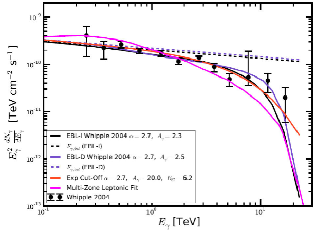
Figure 4 Fit to the observed flux of April 2004 flare with the photohadronic model using two different EBL models are shown. It is also compared with the power-law with exponential cut-off without EBL correction fit ^[38] and with the multi-zone leptonic fit [¹⁶]. The multi-zone leptonic model accounts for the attenuation of the very high energy gamma-rays by the diffuse infrared background. The intrinsic fluxes for both the EBL models are also shown. 

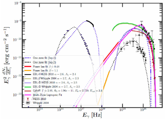
Figure 5 The SED of lep-2 ^[79] is shown along with the powerlaw fit to the SSC tail region with β = 1.1. The best fit to the flare of 2010 using EBL-D and EBL-I are also shown. For comparison, we have also shown the SED of lep-1, the power-law fit to the SSC tail region with β = 0.48 and the best fit to the flare data of 2004 by Whipple telescope ^[16]. The low energy observed data are taken from ref. ^[16,79]. 

In the low energy regime, the lep-1 fit flux increases drastically but this behavior is absent with the lep-2 fit. It is to be noted that, lep-1 corresponds to the observation during the year 2003-2004 and lep-2 is the recent one of January 2013. So we believe that during each observation period, the photon density distribution in the jet changes and this change in the seed photon changes the spectral behavior of the observed multi-TeV gamma-rays. This implies almost simultaneous observation in multiwavelength is essential to fit the observed data. A minor difference between EBL-D and EBL-I predictions for 0.6TeV ≤ E _γ ≤ 20 TeV is observed for 2010 flare data as shown in Fig. 6 and the intrinsic flux is F_γ,in α F^-07_γ Comparison of the intrinsic flux F_γ,in of 2004 and 2010 multi-TeV flaring shows that different spectral shape of the observed events are solely due to the diversity in the shape of the seed photon density distribution (particularly in the SSC tail region) during different epochs.

Figure 6 Fit to the observed flux of 2010 flare by HESS using photohadronic model and EBL correction to it by EBL-D and EBLI are shown. The corresponding intrinsic fluxes are also given. 

4.2 Markarian 501

Markarian 501 (RA:251.46°, DEC:39.76°) is one of the brightest extragalactic sources in X-ray/TeV sky ^[43] and also the second extragalactic object (after Mrk 421) identified as VHE emitter by Whipple telescope in 1996. Since its discovery, the multiwavelength correlation of Mrk 501 has been studied intensively and during this period it has undergone many major outbursts on long time scales and rapid flares on short times scales mostly in the X-rays and TeV energies ^[80-90]. In the year 2009, Mrk 501 was observed as a part of large scale multiwavelength campaign covering a period of 4.5 months (from March 9 to August 1, 2009) ^[63]. The scientific goal of this extended observation was to collect a simultaneous, complete multifrequency data set to test the current theoretical models of broadband blazar emission mechanism. Between April 17 to May 5, this HBL was observed by both space and ground based observatories, covering the entire electromagnetic spectrum even including the variation in optical polarization ^[63]. A very strong VHE flare was detected on May 1st first by Whipple telescope and 1.5 hours later with VERITAS. Both of these telescopes continued simultaneous observation of this VHE flare until the end of the night and the detected flux was enhanced by a factor of ∼ 10 above the average baseline flux. Also a dramatic increase in the flux by a factor ∼ 4 in 25 minutes and a falling time of ∼ 50 minutes was observed. The flux measured at lower energies before and after the VHE flare did not show any significant variation. But, Swift-XRT (in X-ray) and UVOT (in optical) did observe moderate flux variability ^[63]. Using the one-zone SSC model, the average SED of this multiwavelength (up to second peak) campaign of Mrk 501 is interpreted satisfactorily ^[63].

The very strong VHE flare data of May 1st observed by Whipple telescope and the long outburst observed by HEGRA telescopes in 1997 were modeled using the photohadronic model of Ref.^[39]. The model of Dominguez et al. ^[46] is used to correct for the EBL effect on the observed data. Here we shall discuss about the fit to this flare data by different models. To explain the VHE flare of May 1st, 2009, we use the parameters of the one-zone leptonic model ^[63] whose parameters are shown in Table II.

Table II The parameters (up to B’) are taken from the one-zone synchrotron model of Ref. ^[63] which are used to fit the SED of Mrk 501. The last two parameters are obtained from the best fit to the observed Whipple high state flare data from Ref. ^[39]. 

Parameter	Description	Value
MBH	Black hole mass	(0.9 - 3.5) x 109 Mʘ
z	Redshift	0.034
Γ	Bulk Lorentz Factor	12
D	Doppler Factor	12
R’b	Blob Radius	1.2 x 1016 cm
B’	Magnetic Field	0.03 G
R’f	Inner blob Radius	5 x 1015 cm
α	Spectral index	2.4

The observed VHE flare of May 1st was in the range ∼ 317 GeV ≤ E_γ ≤ 5 TeV. In the present context, the above range of E_γ corresponds to the Fermi accelerated proton energy in the range 3.2 TeV ≤ E_p ≤ 50 TeV which interacts with the inner jet background SSC photons in the energy range 13.6 MeV(3.29 x 10²¹ Hz) ≥ ϵ_γ ≥ 0.86 MeV(2.1 x 10²¹ Hz) and finally produce the observed VHE photons. The range of ∈_γ lies in the beginning of the SSC spectrum. A very good fit to the data is obtained for α = 2.4 and A_γ = 89 in in Eq. (19). For comparison we have fitted the data with an exponential cut-off function (dashed dotted curve) and the best fit is obtained for α = 2.6, E_c = 30 TeV and A_γ = 66. Also we have shown the Whipple fit (dashed curve) for comparison, where it is fitted by the function dN_γ /dE_γ = 9.1 x 10^-7 (Eγ/1TeV)^-2.1 ph m^-2s^-1TeV^-1. It is observed that the EBL correction to the VHE γ-ray is small but not insignificant (black curve in Fig. 7) which has a faster fall above 10 TeV. The Whipple data fit very well with the above three scenarios. However, above 5 TeV, both the the EBL corrected fit and the exponential fit differ from the Whipple fit. Again the EBL fit and the exponential fit differ above 10 TeV and the former one falls faster than the latter as clearly shown in Fig. 7. Even though all these fit very well with the Whipple data, deviation is obvious in the VHE limit. Again, between March 16th and October 1st, 1997, Mrk 501 was in a flaring state which was monitored in TeV γ-rays with the HEGRA stereoscopic system of imaging atmospheric Cherenkov telescopes (IACTs). During this long outburst period (a total exposure time of 110 h) more than 38,000 TeV photons were detected and the energy spectrum of the source was above 10 TeV. A time-averaged energy spectrum of this observation period was fitted with a power-law accompanied with an exponential cutoff ^[89]. The same data was reanalyzed with an improved energy resolution ^[90] and found that except for the highest energy, the two analysis were in very good agreement. At the highest energy the spectrum was found to be much steeper than the conventional analysis. In Fig. 7, along with the 2009 flare spectrum, we have also shown the conventional analysis and the improved energy resolution analysis of the 1997 outburst observed by HEGRA telescopes. The photohadronic model of Ref. ^[39] fits very well with the reanalysis result of 1997 flare data beyond 10 TeV. The entire SED (from low to VHE) is shown in Fig. 8 and the intrinsic flux (red curve in Fig. 7) is plotted to show the EBL contribution.

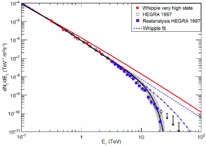
Figure 7 The black curve is the hadronic model fit which includes the EBL attenuation using the EBL model of Dominguez et al. ^[46] to the Whipple very high state flare data (red filled circles) of Mrk 501 and the red continuous curve is the intrinsic flux in the same model. For comparison we have also shown the Whipple fit to the data (dashed curve) and the exponential fit (dashed dotted curve). We have also shown the HEGRA observation of the outburst during 1997: conventional analysis (open circles) ^[89] and new analysis with improved energy resolution (blue filled squares) [⁹⁰]. The shedded region is the region of uncertainty in the EBL model. 

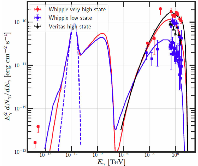
Figure 8 The average SED of Mrk 501 is shown in all the energy bands which are taken from Ref. ^[63]. The SED of low state (MJD 54936-54951; blue squares) and high state (MJD 54952-55; red circles) of the 3-week period are shown. The leptonic model fit to the low state (blue curve) and high state (red curve) are also shown. The blue dotted curve corresponds to the optical emission from the host galaxy. The black curve is the photohadronic fit to the Whipple very high state data (red circles). 

By comparing different time scales and the Eddington luminosity (as done for Mrk 421), the optical depth is in the range 0.04 < τ_pγ < 0.13 and this corresponds to the range of photon density in the inner jet region as 1.5 x 10¹⁰ cm^-3 < n'_γ,f < 5.1 x 10¹⁰ cm^-3. Due to the adiabatic expansion of the inner jet, the photon density will be reduced to n'_γ and also the optical depth τ_pγ << 1. This will drastically reduce the Δ-resonance production efficiency from the ργ process.

4.3 1ES1959+650

The AGN 1ES 1959+650 (z = 0.047) was first detected in the Einstein IPC Slew Survey [⁹¹] and classified as a HBL subclass, based on its X-ray to radio flux ratio with a luminosity distance of d_L =210 Mpc and the mass of the central black hole is estimated to be ∼ 1.5 x 10⁸ M_ʘ. In 1998, VHE gamma-ray from 1ES 1959+650 was observed by the Seven Telescope Array in Utah and later on other observations were also reported. In May 2002, 1ES 1959+650 had a strong TeV outburst which was observed by Whipple ^[13] and HEGRA experiments ^[14] as well as in the X-ray range by RXTE experiments. The X-ray flux smoothly declined throughout the following month. However, during this smooth decline period, a second TeV flare was observed after few days (on 4th of June) of the initial one without a X-ray counterpart [¹⁵]. As this flare was not accompanied by low energy counterparts, it is called orphan flare. So the observation of the orphan flare in 1ES 1959+650 is in striking disagreement with the predictions of the leptonic models thus challenging the SSC interpretation of the TeV emission. Similar behavior also observed in the flare of April 2004 from Markarian 421. Non observation of a significant X-ray activity could naturally be interpreted by the suppression of electron acceleration and inverse Compton scattering as production mechanism for very high energy (VHE) gamma rays in favor of alternative scenarios. To explain the orphan flare, A hadronic synchrotron mirror model was proposed by Böttcher ^[93] to explain this orphan TeV flare from 1ES1959+650 ^[94]. In this model, the flare is explained through the decay of neutral pions to gamma rays when the former are produced due to the interaction of high energy cosmic ray (HECR) protons with the primary synchrotron photons that have been reflected off clouds located at a few pc above the accretion disk. These photons are blue shifted in the jet frame so that there will be substantial decrease in the HECR proton energy to overcome the threshold for Δ-resonance and, at the same time, it is an alternative to the standard scenario where HECR protons interact with the synchrotron photons, where one needs HECR protons to be Fermi accelerated to very high energy. However, how efficiently these photons will be reflected from the cloud is rather unclear.

The SED of the 1ES1959+650 is fitted quite well with the leptonic one-zone synchrotron and SSC model ^[95,96]. In all these models, although the blob size differ by about 1 to 2 orders of magnitudes (1.4 x 10¹⁴ cm ≤ R'_b ≤ 1.4 x 10¹⁶ cm), the bulk Lorentz factor Γ and D are almost the same (18 ≤ Γ ≃ D ≤ 20). The multiwavelength observation of 1ES 1959+650 was performed in May, 2006 and the SED fitted with the above one-zone model by Tagliaferri et. al [⁹⁵], for which the parameters used are Γ ≃ D = 18, R'_b = 7.3 x10¹⁵ cm and B’ = 0.25 G. To explain the VHE spectrum of the orphan flare in photohadronic model ^[35], Γ = 18 is also used.

The observed flare energy was in the range 1.26TeV(3.05 x 10²⁶Hz) ≃ 9.4TeV(2.3 x 1027Hz). Gamma-ray in this energy range is produced when protons in the energy range 12 TeV ≤ E_p ≤ 94 TeV collide with the background photons in the energy interval 7.5 MeV(1.8x10²¹Hz) ≥ ϵ_γ ≥ 1MeV(2.4x10²⁰ Hz). The range of ∈γ lies exactly in the low energy tail of the SSC photons as shown in Fig. 9, calculated using the one-zone leptonic model and flux in this region also has a power-law behavior Φ_SSC ∝ϵγβ. As discussed for Mrk 421 and Mrk 501, we can relate the photon density in the inner region to the outer region and calculate the observed high energy flux.

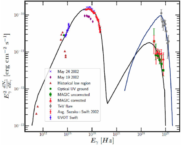
Figure 9 The multiwavelength SED measured at the end of 2006 May with other historical data from Ref. [⁹⁵] are shown. Different symbols are observations with different sources marked within the box, and the curves are model fits: The curve (from low energy to high energy) is synchrotron + SSC fit from Tagliaferri et. al. ^[95], while the second curve (extreme right) is the photohadronic fit to the flare data. 

Best fit to the observed VHE spectrum is obtained with the values of α =2.83 and E_c = 4.2 TeV ^[14] for power-law with exponential cut-off. The γ-ray cut-off energy of 4.2 TeV corresponds to E_p,c = 42 TeV and above the cut-off energy the flux decreases. For power-law with EBL correction, the best fit is obtained for α = 2.8 and Aγ = 87 (black curve) using Eq. (19). For comparison, both the exponential and the EBL fits are shown in Fig. 10. The exponential fit falls faster than the EBL fit above 16 TeV. The time averaged TeV energy spectrum (above 1.4 TeV) of the flaring state of the 1ES 1959+650 was well fitted with pure power-law by the HEGRA collaboration and the power-law spectral index is α=2.83±0.14_stat±0.008_sys or by a power-law with an exponential cut-off at E_c = (4.2^+0.8_-06stat ± 0.9_sys) TeV and a spectral index of 1.83±0.15_stat±0.08_sys [^14,97].

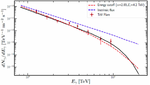
Figure 10 The flare data are fitted with power-law with exponential decay (red dotted curve) and power-law with EBL correction (black curve). The blue dotted curve is the intrinsic flux. 

In Fig. 9, the flare data is shown along with the fit. Normally, it is observed that the flux increases for Eγ = 1.2 TeV due to the high proton flux in this energy range. However, in order not to violate the Eddington luminosity, the proton energy spectrum must break to a harder index (e. g.α ∼ 2.3) below 12 TeV. So a break in proton spectrum is introduced at E_p,b ∼ 12 TeV below which α = 2.3 and above this energy α = 2.8 so that the gamma-ray flux falls below 12 TeV.

5. General Remark

A general discussion of shortcomings in different models is discussed here. In proton synchrotron models ^[55], the interaction of high energy protons with the synchrotron photons in the jet can produce γ-rays from π⁰ decay and can explain the multi-TeV emission from blazars. Also Zdziarski et al. ^[98,99] have used the hadronic model to explain the broad band spectra of radio-loud AGN. These scenarios require super Eddington luminosity in protons (∼ 10⁶ times the Eddington flux) to explain the multi-TeV emission. Also, synchrotron emission from the ultra high energy protons in the jet magnetic field can explain the VHE γ-ray SED ^[68] but strong magnetic field at the emission site is a necessary requirement which is probably not there. In an alternative scenario, ultra high energy protons escaping from the jet region produce VHE photons by interacting with the cosmic microwave background (CMB) photons and/or EBL which avoids the absorption in the inner jet region ^[100]. This explains the transparency of the universe to VHE γ-rays due to their proximity to the Earth compared to the one produced in the source which travels a longer distance. Also the TeV spectrum is independent of the intrinsic spectrum but depends on the output of the high energy cosmic rays in the source. This model fits very well to multi-TeV spectra from many sources ^[69,101-103]. However, in this scenario, it is assumed that the source produces VHE protons with energies 10¹⁷ - 10¹⁹ eV (this is true with most of the hadronic models) and a weak extragalactic magnetic field in the range 10^-17 G < B <10^-14 G is needed. So far we have not observed either high energy cosmic ray event or high energy neutrino event from nearby HBLs (e.g. Mrk 401, Mrk 501 etc.) when they were flaring and also the extragalactic magnetic field seems to be weak. However, in the photohadronic model discussed above, ργ→Δ process takes place in the hidden inner jet region where the photon density is order of magnitude higher than the normal jet and overcomes the super-Eddington energy budget. Also, the energy of the Fermi accelerated proton is E_p = 10Eγ which can be achieved easily in the jet.

Normally it is difficult to explain the GeV-TeV emission from HBLs through one-zone leptonic model. On the other hand, multi-zone leptonic models overcome this problem and explain the multi-TeV data but one has to increase the number of parameters. A power-law with an exponential cut-off energy E_c is the conventional method used in the literature to explain the exponential fall of the multi-TeV flare from flaring blazars where the free parameter E_c depends on some unknown mechanism. The EBL correction does the same job as the exponential decay factor. So the inclusion of EBL effect eliminates the necessity of the extra parameter E_c.

The high energy protons will be accompanied by high energy electrons and these electrons will emit synchrotron photons in the magnetic field of the jet. The energy range of the photons emitted lie in between the high energy end of the synchrotron spectrum and the low energy tail of the SSC spectrum, thus may not be observed due to their low flux in this region. The secondary charged particles e^±, π^±, μ^± produced within the jet will also emit synchrotron photons and their energy will be much smaller than the synchrotron photons produced from the primary electrons accompanying the high energy protons. So even though the charged particles emit synchrotron radiation, their contribution will be small.

The problem with the photohadronic model is that, the gamma-rays are produced from the pion decay within the inner jet region where photon density is very high compered to outer region. So γγ → e⁺e^- should be efficient, which will attenuate the propagation of multi-TeV gamma-rays from the production site. However, observation of multi-TeV gamma-ray events from many flaring HBLs observed by MAGIC, VERITAS, HESS telescopes guarantees that gamma-rays do escape from the jet without undergoing pair production, so the pair production process can be constrained. The photohadronic model works well for high energy gamma-rays (above ∼ 100 GeV), so in the lower energy regime, it is the leptonic model which contributes to the multiwavelength SED. In principle both should coincide at some intermediate energy.

6. Summary

One-zone leptonic model is very successful to explain the synchrotron and SSC peaks of AGN. But this model has difficulties to explain the multi-TeV emission/flaring from many HBLs. In this article, we review the photohadronic model which is very successful to explain the multi-TeV flare data from the nearest HBLs Mrk 421, Mrk 501 and 1ES1959+650. As high energy gamma-ray is attenuated by the EBL, it is necessary to account for it which is considered here and compared with the exponential cut-off scenario and other power-law fits. The main objective here is to understand the flaring from nearby HBLs so that the mechanism to produced intrinsic flux can be understood well and also it can be useful to understand the flaring from far off HBLs. This model uses the leptonic model parameters which explains the first two peaks of the AGN very well as input. In the photohadronic scenario, the observed flux is proportional to the SSC flux Φ_SSC which is a power-law, Φ_SSC ∝Eγ-β in the lower tail region. Then, measurement of SSC flux in the low energy tail region is required. But, most of the cases this region of the SED is not observed/measured due to technical difficulties. Hence, model calculations are used for it and different models give slightly different β. As the photohadronic model depends on Φ_SSC , simultaneous multiwavelength observation of the object during the flaring is important and in few cases it has already been done. In future, accurate measurement of EBL contribution and observation of HBLs above 30 TeV energy range will definitely constrain severely different models discussed above.