Analytical solution of the bioheat equation for thermal response induced by any electrode array in anisotropic tissues with arbitrary shapes containing multiple-tumor nodules

Roca Oria, E. J.; Bergues Cabrales, L. E.; Bory Reyes, J.; Roca Oria, E. J.; Bergues Cabrales, L. E.; Bory Reyes, J.

doi:10.31349/revmexfis.65.284

Servicios Personalizados

Revista

Articulo

Indicadores

Citado por SciELO
Accesos

Links relacionados

Similares en SciELO

Otros
Otros

Permalink

Revista mexicana de física

versión impresa ISSN 0035-001X

Rev. mex. fis. vol.65 no.3 México may./jun. 2019 Epub 30-Abr-2020

https://doi.org/10.31349/revmexfis.65.284

Research

Analytical solution of the bioheat equation for thermal response induced by any electrode array in anisotropic tissues with arbitrary shapes containing multiple-tumor nodules

E. J. Roca Oria^a

L. E. Bergues Cabrales^b^*

J. Bory Reyes^c

^{^a}Departamento de Física, Facultad de Ciencias Naturales y Exactas, Universidad de Oriente, Santiago de Cuba, Cuba.

^{^b}Departamento de Ciencia e Innovación, Centro Nacional de Electromagnetismo Aplicado, Universidad de Oriente, Santiago de Cuba, Cuba.

^{^c}ESIME-Zacatenco, Instituto Politécnico Nacional, CDMX, México.

Abstract

The Pennes bioheat transfer equation is the most used model to calculate the temperature induced in a tumor when physical therapies like electrochemical treatment, electrochemotherapy and/or radiofrequency are applied. In this work, a modification of the Pennes bioheat equation to study the temperature distribution induced by any electrode array in an anisotropic tissue containing several nodules (primary or metastatic) with arbitrary shape is proposed. For this, the Green functions approach is generalized to include boundaries among two or more media. The analytical solution we obtain in a very compact way, under quite general assumptions, allows calculating the temperature distributions in the tumor volumes and their surfaces, in terms of heat sources, initial temperature and calorific sources at the boundary of tumors.

Keywords: Bioheat equation; Green function; electric field; electric current density; tumor anisotropy

PACS: 34B27; 35K05; 80A20; 92C05; 92C50; 97M60

1. Introduction

Therapies like electrochemical treatment (EChT) ^[1], electrochemotherapy (ECT) ^[2] and radiofrequency ablation (RF) ^[3] have emerged as safe and effective treatments for solid tumors with minimum damage to the organism. During application of these therapies, tissue heating arises due to conduction losses (i.e., resistive heating from ion movement) ^[4]. Thermal spread in biological tissue may be measured using an infrared thermograph device ^[5]. Images of surface temperature and false-positive and false-negative constitute limitations of the infrared thermography method ^[6,^7]. Therefore, several researchers have addressed their efforts to know how the temperature is distributed in a tissue (i.e., the tumor) ^[8-^10]. Furthermore, mathematical modeling is used ^[8,¹¹-^13]. These studies evidence that thermal modeling is more complex than electrical ones because diffusion process depends on time. Heat transfer has an important role in biological systems of living beings ^[11,¹⁴,^15]. The Pennes bioheat equation is crucial for the majority of the bioheat transfer simulations ^[16]. It has been used when the internal heat generation of tissue is produced by its metabolism ^[17]. Additionally, Pennes bioheat equation permits to describe the energy conservation equation for biological heat transfer on the basis of the classical Fourier’s law of heat conduction ^[5]. Analytic modeling of temperature distribution is based on solving the linear bioheat transfer equation for tissue, which is the general heat equation for conduction, with added terms for heat sources ^[8-¹⁰,^18].

Pennes bioheat equation has been previously used to model temperature distribution in non-homogenous tissues ^[11,¹⁹,^20], in which heat sources (one or several electrodes) are inserted. Gupta et al. ^[21] make a numerical study on heat transfer in tissues for different coordinate systems and under different boundary conditions (first kind, second kind and third kind). They conclude that during thermal therapy, probe shape, boundary conditions and internal heat source should not be the same and must be changed from one organ to the other in the human body.

Kumar et al. ^[22] report that treatment of cancerous cell is independent of the generalized coordinate system considered at the thermal ablation position. Additionally, Pennes bioheat equation has been used to describe the heat transfer for targeted brain hypothermia, which is a result of the decreasing arterial blood temperature ^[23].

We are not aware on applications of the bioheat equation for two media (tumor and the surrounding healthy tissue) with different biological, electrical (electrical conductivity and electrical permittivity), mechanical and thermal properties, as reported in ^[24,^25]. Besides, the thermal treatment of several tumor nodules in tissue/organism simultaneously has not been reported in the literature.

In this study, a modification of the linear bioheat equation is proposed to calculate the temperature in a multi-centric tumor and the surrounding healthy tissue, considering them as linear, heterogeneous and anisotropic media of arbitrary shapes. Besides, in this generalized equation the thermal, electrical, mechanical and biological properties of each biological tissue are considered.

2. Theory

2.1 Model assumptions

Heat transfer among the tumors occupying the regions Vi(i=1,2,…,N) with surfaces boundaries Si (i=1,2,…,N) and the surrounding healthy tissue (region to be denoted by V0) can be modeled by the bioheat transfer equation ^[10] governing the temperature distribution, T=T(r⃗,t) in Kelvin, which is given by

ρc∂∂tT=∇⋅(k↔⋅∇T)+j→⋅E→-ρbωbcb(T-Tb)+Q(r→,t), (1)

where t is the time, for each r⃗∈V:=∪i=0NVi. A schematic representation of V0, Si and Vi is shown in Fig. 1. The parameters (in general, different in each medium) ρ (kg/m3) and c (J/kg K) are the mass density and the specific heat of each tissue, respectively. In general, thermal conductivity k↔ (W/m K) is a real symmetric tensor of second order. j⃗(r⃗,t) (A/m2) and E⃗(r⃗,t)(V/m) are the fields of current density and electric field intensity, respectively. j⃗⋅E⃗ is the Joule heating term.

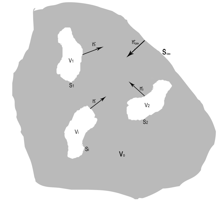
FIGURE 1 Schematic representation of work region: V0 is the region that occupy the surrounding healthy tissue and contain several tumors of different sizes Vi(i = 1; : : : ;N), where Vi is the -th tumor volume and N is the amount of tumors. Parameters Si (i = 1; 2; : : : ;N) and S1 represent surface boundaries and surface very far from the tumors, respectively. Besides, n→i is the normal unit vector to the surface Si directed to media Vi and n→∞ (coincides with Vi and n→0) is the normal unit vector directed to medium V0.

Although the heat sources are in the tumors, Joule heating terms are different on each tissue. The parameter Q(r⃗,t) is the metabolic heat in the tumors and their surrounding healthy tissues. These metabolic heats are different because the metabolic processes that happen in these tissues are different ^[24]. The term -ρbωbcb(T-Tb) represents a heat source due to blood circulation ^[12]. Tb is the temperature of the arterial blood. ωb, ρb and cb are the perfusion, density and the specific heat of blood, respectively. ωb, ρb, cb and Tb are considered constant in each tissue. When T be referred to regions Vi, we will use denotation T(i)(i=1,…,N).

The electric potential Φ can be calculated assuming biological tissues as linear, i.e., it is j⃗=σ↔⋅E⃗ (Ohm’s law), where σ↔ is the electric conductivity tensor. Moreover, combining quasi-static approximations (0=∇⋅j⃗+∂ρ/∂t≈∇⋅j⃗ and E⃗=-∇Φ), under Ohm’s law, we obtain

∇⋅⌊σ↔-1∇Φ⌋=0. (2)

The Joule heat is calculated by means of j⃗⋅E⃗=∇Φ⋅σ↔⋅∇Φ. Rigorously, Eqs. (1) and (2) are coupled linear equations because the electric conductivity depends on the temperature ^[10] but in this paper this dependence is disregarded. For a recent account of the problem for different electrode configurations we refer the reader to ^[10,¹⁸,^26].

In this study, Eq. (1) is addressed to EChT, although it can be indistinctly used for EChT, ECT or RF. In this case, j⃗⋅E⃗ is due to the electrodes inserted completely in the tumor ^[27,^28].

Let us denote the initial distribution of T in all media by

T(r⃗,0)=:T0(r⃗). (3)

It is important to assess T0(r⃗) in Eq. (3) because T0(0)(r⃗)≠T0(i)(r⃗) (i=1,2,…,N), generally due to inflammatory and others processes that occur in unperturbed tumors ^[24]. In the first approximation, it can be considered that T0(r⃗)=Tb=36.5 ∘C, which is the body temperature. Indeed, in preclinical ^[28] and clinical ^[27] studies, it has been reported that the regions away from the tumors are not damaged by EChT action, when the electrodes are completely inserted into the tumor. Besides, neither Tb nor the blood vessels are affected during or after EChT application.

Matching boundary conditions on the surfaces Si that separates the tumors of the surrounding healthy tissue are

r→∈Si(i=1,2,…,N):{T(i)(r→,t)=T(0)(r→,t),r→i⋅(k↔i⋅∇T(i))+r→0⋅(k↔i⋅∇T(0))=-q (4)

where n⃗i and n⃗0 are both normal unit vectors to the surface Si but directed to media Vi and V0, respectively (Fig. 1). The parameter q is the surface energy density generated by the metabolic processes that may be related with the exchange of nutrients, substances, energy, information between the tumor and the surrounding healthy tissue ^[24].

Finally, the temperature distribution at points away from the tumors satisfies the following condition

r→∞:T(0)(r⃗,t)→Tb. (5)

Considering the above-mentioned assumptions and the change of variables T(r⃗,t)-Tb→T(r⃗,t), Eq. (1) can be rewritten

ρc∂∂tT=∇⋅(k↔i⋅∇T(0))-λT+f(r⃗,t), (6)

With

λ=ρbωbcb, (7)

f(r⃗,t)=j⃗(r⃗)⋅E⃗(r⃗)+Q(r⃗,t) (8)

To deal with T0(0)(r⃗)=T0(0)(r⃗)=Tb, (i=1,2,…,N), we note that Eq. (3) is reduced to

T(r⃗,0)=0. (9)

Note that Eq. (4) is not altered and Eq. (5) adopts the form

r→∞:T(0)(r⃗,t)→0. (10)

2.2 Green Functions

As Eq. (4) (matching boundary conditions) and Eq. (6) are not homogeneous, let us introduce the Green functions of the problem for the tumors and the surrounding healthy tissue Gl(r⃗,t,r⃗l,t') (l=0,1,…,N). Indeed, we have

ρc∂∂tGl=∇⋅(k↔⋅∇Gl)-λGl+δ(r→-r→l)δ(t→-t→'),r→l∈Vl(l=0,1…,N) (11)

The independent term δ(r⃗-r⃗l)δ(t⃗-t⃗') in Eq. (11) corresponds to the effect of a unit source located at the point r⃗l and at the time instant t', upon the point r⃗ at the time instant t. Note that there appear N+1 Green functions, one for each parameter r⃗l∈Vl(l=0,1…,N).

Usually, the Green function is employed in the solution method of the Dirichlet boundary problem and Neumann boundary problem (normal derivative specified on the boundary). In the present model, Dirichlet and Neumann conditions are substituted by matching boundary conditions. So, the usual approach must be changed: the initial condition and matching boundary condition for Eq. (11) are

Gl(r⃗,t,r⃗l,t')=0, t<t', (12)

r⃗∈Si(i=1,2,…,N):*20cGl(0)(r⃗,t;r⃗l,t')=Gl(i)(r⃗,t;r⃗l,t'),n⃗0⋅(k↔0⋅∇Gl(0)(r⃗,t;r⃗l,t'))+n⃗i⋅(k↔i⋅∇Gl(i)(r⃗,t;r⃗l,t'))=0, (13)

2 for l=0,1…,N.

The condition at infinity is not changed:

r→∞:Gl(0)(r⃗,t;r⃗l,t')→0. (14)

If T'(r⃗,t) satisfies the same problem as T(r⃗,t) except for q̃ and f̃ instead of q and f, respectively, then T̃(r⃗,t):=T'(r⃗,-t) satisfies the adjoint equation of Eq. (6)

ρc∂∂tT̃=∇⋅(k↔i⋅∇T̃)-λT̃+f̃, (15)

and the same boundary conditions for T(vecr,t) (see Eq. (4)) but with q̃ instead of q. Also, assuming Eq. (10) holds in the sense

r→∞:*20crT→0,rT̃→0, (16)

we can proceed in the following way: multiplying Eq. (6) by T̃, as well as Eq. (15) by T and subtracting the obtained equations, we get

ρc∂∂t(TT~)=T~∇⋅(k↔⋅∇T)-T∇⋅(k↔⋅∇T~)+fT~-f~T.f~, (17)

Considering the vector identity (see Eq. (9) in ^[29])

∇⋅(φψ⃗)=∇φ⋅ψ⃗+φ∇⋅ψ⃗, (18)

with ψ⃗=k↔⋅∇T and ψ⃗=k↔⋅∇T̃, it is obtained

∇⋅(T~k↔⋅∇T-Tk↔⋅∇T~)=∇T~⋅(k↔⋅∇T)+T~∇⋅(k↔⋅∇T)-T∇⋅(k↔⋅∇T~), (19)

because ∇T̃⋅(k↔⋅∇T)=∇T⋅(k↔⋅∇T̃) because k↔ is a real symmetrical tensor.

Applying the divergence theorem to Eq. (19), we deduce that

∫VdV∇⋅(T~k↔⋅∇T-Tk↔⋅∇T~)=∮SdS→⋅(T~k↔⋅∇T-Tk↔⋅∇T~)+∫S∞S→⋅(T~k↔⋅∇T-Tk↔⋅∇T~)d, (20)

where S∞ is a surface very far from the tumors (Fig. 1) and dS⃗=n⃗⋅dS. The integral extended to S∞ vanishes, supposing condition (16). Indeed,

r→∞:[T∼1r,n→⋅∇T~∼∂∂tT~∼1r2]⇒Tn→⋅∇T~dS=1r→0.

The integral extended to S=∪i=1NSi may be calculated by using boundary conditions for T (Eq. (4)) and T̃ (see line after Eq. (15)):

∮SdS→⋅(T~k↔⋅∇T-Tk↔⋅∇T~)=-∑l=1N∮Sl×[T~(l)(n→l⋅k↔l⋅∇T(l)+n→0⋅k↔0⋅∇T(0))-T(l)(n→l⋅k↔l⋅∇T~(l)+n→0⋅k↔0⋅∇T~(0))=∮SdS(T~q-Tq~). (21)

The minus sign in the integrals is explained because Maxwell normal is opposite to that of Gauss.

Integrating Eq. (17) and using Eqs. (20) and (21) yields

∫VVρc[TT~]t=t2t=t2d=∫t1t2dt∮dS(T~q-Tq~)+∫t1t2dt∫dV(T~f-Tf~), (22)

where t1>0 and t2>0 and arbitrarily selected.

Note that, according to the definition of T̃(r⃗,t) and comparing Eq. (15) with Eq. (11) we get the definition of G̃

G̃j(r⃗,t;r⃗j,t″)=G̃j(r⃗,-t;r⃗j,-t″). (23)

Therefore, initial condition (12) implies that

G̃j(r⃗,t;r⃗j,t″)=0, t>t″. (24)

Two direct consequences follow from Eq. (22): the reciprocity principle

G̃j(r⃗l,-t';r⃗j,-t″)=G̃j(r⃗j,t″;r⃗l,t'), (25)

and the formula

T(r→j,t')=∫0t'+ηdt∫VdVG~j(r→j,t';r→,t)f(r→,t)+∫VdVρcG~(r→j,t';r→,0)T(r→,0)+∫0t'+ηdt∮SdSG~j(r→j,t';r→,t)q(r→,t). (26)

The reciprocity principle (25) means that the influence in (r⃗j,t″) of a unit source, placed in (r⃗l,t'), is the same as that (r⃗l,-t') of the same source at (r⃗j,-t″).

The Eq. (26) evidences that T in all media can be calculated from the superposition of the following contributions: heat sources f of Eq. (8) (first term), initial temperature (second term) and calorific sources q at the boundary of tumors (third term). The interpretation of the first term agrees with the physical meaning of Green function: the response of a unit impulse must be multiplied by the intensity f and then superposed to all points of the media from the instant of time in which the source is turned on (compare with Eq. (7.4.9) for a single medium ^[30]). The physical sense of the last two terms of Eq. (26) is similar. Note that anisotropy and inhomogeneity of the media appear only in each Green function.

The proof of Eq. (25) is completed by taking T(r⃗,t)=Gl(r⃗,t;r⃗l,t') and T̃(r⃗,t)=G̃j(r⃗,-t;r⃗j,-t″), in Eq. (22). The surface integral is zero because q̃=q=0. Choosing t1=0 and t2>t',t2>t″, Eqs. (12) and (24) are sufficient to guarantee that the left member of Eq. (22) is zero too. Finally, by the fundamental property of the Dirac delta function we have

∫VdVf(r⃗)δ(r⃗-r⃗')=f(r⃗'),

and Eq. (25) follows, which is clear from Eq. (22).

Equation (26) follows using Eq. (24), Eq. (25), the fundamental property of delta function and substituting,T̃(r⃗,t)=G̃j(r⃗,-t;r⃗j,-t') t1=0 and t2=t'+η(η>0) into Eq. (22).

The second term of Eq. (26) is zero because of Eq. (9). As a result, Eq. (26) can be rewritten as

T(r→j,t')=∑l=0N∫0t'+ηdt∫VidVlGl(r→j,t';r→l,t)f(r→l,t)+∑l=0N∫0t'+ηdt∮SdSlGl(r→j,t';r→l,t)q(r→l,t), (27)

for every η>0 and j=0,1,…,N.

We set t2=t'+η(η>0) to guarantee that the upper limit of t' does not contribute in the second term of the second integral in Eq. (22), which is clear from Eq. (24). It is convenient to choose t1=0 such that t' could be selected by the Dirac delta function in the integral of the left member of Eq. (22).

The desired solution T in terms of Green functions is given by Eq. (27), which depends on contributions of caloric sources inside the media (Eq. (8)) and on the boundary (Eq. (4)).

2.3 Calculation of the Green functions by means of eigenfunctions

From Eq. (27), the required solution is given in terms of the complementary conditions of the formulated problem, if Green functions are known. An usual method to calculate these functions consists in expanding them in terms of eigenfunctions of the operator L^:=-∇⋅(k↔⋅∇) defined in the Hilbert space H=L2(V) of square-integrable functions in V=∪i=0NVi with scalar product (ψ,φ):=∫VdVψ¯φ where ψ¯ is the complex conjugate function of ψ.

Assuming the following boundary conditions:

r→∈Si(i=1,2,…,N):{φ(i)(r→)=φ(0)(r→),n→i⋅(k↔i⋅∇φ~(i))+n→0⋅(k↔0⋅∇φ~(0)) (28)

r→+∞:φ(2)≈1r, (29)

the domain of L^ will be

D(L^):={φ∈H/L^φ∈H}, (30)

such that φ satisfies Eqs. (28) and (29)

The analysis relative to Eq. (21) shows that the domains of the operator L^ and its adjoint, denoted by L^+, coincide and that L^ is self-adjoint

D(L^+)=D(L^), L^+=L^. (31)

Besides, L^ is positive (denoted by L^>0) because Eq. (18) implies

ϕ¯L^ϕ=-ϕ¯∇⋅(k↔⋅∇ϕ)=∇ϕ¯⋅(k↔⋅∇ϕ)-∇⋅(ϕ¯k↔⋅∇ϕ). (32)

The scalar product arises from integration of Eq. (32). This brings about that the second term in the right hand side of Eq. (32) be zero, by an analogous calculation to Eq. (21), resulting that

ϕ≠θ⇒(ϕ,L^ϕ)=-∫VdVϕ¯∇⋅(k↔⋅∇ϕ)=∫VdV∇ϕ¯⋅(k↔⋅∇ϕ)>0∴L^>0, (33)

because the tensor is also positive. Hence, the eigenvalues (λn) of L^ are real and positive ^[31],

L^ϕn=λnϕn⇒λn>0.

Note that the eigenfunctions of L^ coincide with those of L^+λ but the eigenvalues are displaced by λ:

(L^+λ)ϕn=L^ϕn+λϕn=(λn+λ)ϕn. (34)

From Eq. (31), it follows also that there is an orthonormal and complete system (ϕn) of H entirely composed of eigenfunctions of L^, which means ^[32]

∀φ∈H:φ=∑nφnϕn, φn=(ϕn,φ). (35)

This permits the calculation of the Green function, given by

G(r⃗l,t',r⃗,t)=∑ngn(t';r⃗,t)ϕn(r⃗l), gn(ϕn,G). (36)

Substituting Eq. (36) in Eq. (11) and using the definition of eigenfunction, yields

∑n[ρc∂gn∂t+(λn+λ)gn]ϕn=δ(r→l-r→)δ(t'-t),r→l∈Vl(l=0,1,…,N). (37)

From Eq. (36) and Eq. (37) results

ρc∂gn∂t+(λn+λ)gn=(ϕn,δ(r→l-r→)δ(t'-t))=δ(t'-t)ϕn(r→). (38)

Suppose ρc be constant in each medium, then the spatial part of Eq. (38) can be separated

gn(t';r⃗,t)=ϕn(r⃗)g̃n(t';t). (39)

to obtain an ordinary differential equation

ρc∂g̃n∂t+(λn+λ)g̃n=δ(t'-t). (40)

The solution of Eq. (40) is given by

g̃n(t';t)≡g̃n(t'-t)=1ρceΛn(t'-t)h(t'-t). (41)

where

Λn=λ+λnρc,h(t'-t)={1,t<t'0,t>t', (42)

Substituting Eq. (41) into Eq. (39) and using the mentioned result in Eq. (36), we obtain the expression of the desired Green function, given by

G(r→l,t',r→,t)=∑ne-Λn(t'-t)ρch(t'-t)ϕn(r→l)ϕ¯n(r→)(l=0,1,…,N). (43)

From Eq. (43), Green functions are zero for t>t', according to the definition of h in Eq. (42), in agreement with the causality requirement (Eq. (12)) for Green function. For t<t', Green function decreases exponentially if the time increases, as it typically happens in the conduction processes.

Note that the structure of Eq. (43) shows that anisotropy and inhomogeneity of media appear only in eigenfunctions.

Substituting Eq. (43) into Eq. (26), one obtains

T(r→l,t',r→,t')=∑nϕn(r→)∫0t'×[∫0dVϕ¯n(r→)f(r→,t)ρc+∮dSϕ¯n(r→)q(r→,t)ρc]e-Λn(t'-t)dt. (44)

3. Remarks on generalized Pennes equation

The formal solution (44) is compact and obtained under quite general suppositions (linearity and ρc constant in each medium anisotropic and heterogeneous). It permits to know how the temperature is distributed in the tumor and in the surrounding healthy tissue when a single tumor appears in the host. Furthermore, this equation can be used to estimate the temperature in a tissue, organ and/or an organism that contains several tumor nodules (primary and/or metastatic) with arbitrary shapes and different histogenic characteristics, unprecedented in the literature. This later gives solution to the suggestion reported in ^[22]. Additionally, thermal influences of both media and their boundaries are included separately in the solution (44), and the contribution of each eigenfunction decreases exponentially in time with its relaxation time Λn-1, which depends on the medium properties (Eq. (42)).

It is interesting to note that the solution (44) allows us to know the temperature distribution in the tumor volume and in its surface separately. Increase/decrease of the temperature gradient between the tumor volume and its surface could be induced. This can be possible by controlling the temperature generated by any geometry of electrode array reported in the literature ^[13,³³-^37] and the blood perfusion in the tumor. These aspects agree with the ideas of Ma et al. ^[23].

On the other hand, the solution (44) is valid for electrodes of any shape ^[36]. Furthermore, this mathematical formalism permits to suggest strategies to treat each nodule individually, depending on its stiffness, histogenic characteristics, shape and electrical properties. The dielectric properties of biological tissues have been published by several researchers ^[4,^38]. Nevertheless, k↔ may be experimentally known from tridimensional anisotropy matrix of biological tissue (tumor and/or the surrounding healthy tissue) using diffusion tensor imaging technique, as reported in ^[39]. Values of components of this matrix depend on tumor histological variety and type of the healthy tissue that surrounds the tumor.

The spatial distributions of the temperature, electric field strength and electric current density may be calculated in a realistic tumor model using finite element methods, taking into account the work of Korshoej et al. ^[40]. Nevertheless, it is suggested for EChT the integrated analysis of the electric potential, temperature, electric field strength, electric current density, pH and tissue damage spatial distributions generated by any geometry of electrode in the tumor and its surrounding healthy tissue, as reported in ^[13,^37]. It is important to note that the antitumor mechanism more accepted in EChT is the induction of toxic products from electrochemical reactions ^[27,²⁸,^36].

In addition to the above mentioned, the solution (44) can be implemented in a numerical algorithm for the simulations. A further study can be carried out to simulate all physical quantities above mentioned and tissue damage in realistic anisotropic media with arbitrary shapes, electrode arrays with different geometry and arbitrary shape of the electrode. As the solution (44) is obtained for constant initial condition, it would be interesting to know how the solution (44) changes when spatially dependent initial condition is used, as reported in ^[5].

4. Conclusions

In conclusion, a general method is developed to calculate temperature distributions in two coupled linear and anisotropic media (solid tumor and the surrounding healthy tissue). This approach can be easily generalized to multi-centric tumors in a tissue or to several tumors (primary or metastasis) in the organism by changing the summation indices. For this propose, the method of Green functions is extended to include matching boundary conditions.

Acknowledgments

Authors thank anonymous referees, Editor in Chief and Yenia Infante Frómeta for their valuable comments and technical assistances. E. R. Oria and L.E.B. Cabrales are supported by grant 9116 from Centro Nacional de Electromagnetismo Aplicado, Universidad de Oriente, Cuba. J.B. Reyes is supported by SIP-program under number SIP-20180225.

References

1. L. E. B. Cabrales et al., BMC Cancer 10 (2010) 1. [ Links ]

2. C. K. Sung et al., Tech. Cancer Res. Treat. 16 (2016) 488. [ Links ]

3. W. Yang, M. Cui, J. Lee, W. Gong, S. Wang, J. Fu, G. Wu, K. Yan, Chin. J. Cancer Res. 28 (2016) 19. [ Links ]

4. D. Haemmerich, B. J. Wood, Int. J. Hyperth. 22 (2006) 563. [ Links ]

5. J. Dutta, B. Kundu, J. Therm. Biol. 66 (2017) 33. [ Links ]

6. P. R. Pavithra, K. S. Ravichandran, K. R. Sekar, R. Manlkandan, Sys. Rev. Pharm. 9 (2018) 10. [ Links ]

7. G. Dua, R. J. Mulaveesala, Biomed. Opt. 23 (2018) 037001. [ Links ]

8. C. S. Daniels, B. Rubinsky, Plos One 6 (2011) e20877. [ Links ]

9. P. A. Garcia, R. V. Davalos, D. Miklavcic, Plos One 9 (2014) e103083. [ Links ]

10. I. Lackovíc, R. Magjarevíc, D. Miklavcic, IEEE T. Dielect. El. In. 16 (2009) 1338. [ Links ]

11. K. Das, S. C. Mishra, J. Therm. Biol. 45 (2014) 103. [ Links ]

12. P. K. Gupta, J. Singh, K. N. Rai, J. Therm. Biol. 35 (2010) 295. [ Links ]

13. A. Soba, C. Suarez, M. M. Gonzalez, L. E. B. Cabrales, A. E. B. Pupo, J. B. Reyes, Math. Compt. Simul. 146 (2018) 160. [ Links ]

14. M. A. Ezzat, N. S. AlSowayan, Z. I. Al-Muhiameed, S. M. Ezzat, Heat and Mass Transfer 50 (2014) 907. [ Links ]

15. M. Shahnazari, C. Aghanajafi, M. Azimifar, H. Jamali, IJRRAS 17 (2013) 1. [ Links ]

16. H.H. Pennes, J. Appl. Physiol. 85 (1948) 5. [ Links ]

17. T. Lillicrap, M. Tahtal, A. Neely, X. Wang, A. Bivard, C. Lueck, Australas. Phys. Eng. Sci. Med. 40 (2017) 841. [ Links ]

18. C. Suarez, , F. Maglietti, N. Olaiz, G. Marshall, Plos One 9 (2015) e113413. [ Links ]

19. T. R. Gowrishankar, D. A. Stewart, G. T. Martin, J. C. Weaver, Biomed. Eng. Online 3 (2004) 42. [ Links ]

20. D. Mitchell et al., Int. J. Hyperther. 34 (2018) 1. [ Links ]

21. , J. Singh , K. N. Rai, Math. Comput. Model. 57 (2013) 1018. [ Links ]

22. D. Kumar, P. Kumar, K. N. Rai, Procedia Eng. 127 (2015) 1300. [ Links ]

23. W. Ma, W. Liu, M. Li, Int. J. Therm. Sci. 100 (2016) 66. [ Links ]

24. R. S. Cotran, V. Kumar, T. Collins, Patología Estructural y Funcional, Sexta Edición, (McGraw-Hill- Interamericana de España, S.A.U., Madrid, 1999), p. 277. [ Links ]

25. D. Hanahan, R. A. Weinberg, Cell 144 (2011) 646. [ Links ]

26. T. Forjanic, D. Miklavcic, Biomed. Eng. Online 17 (2018) 80. [ Links ]

27. C. K. Chou, J. A. McDougall, C. Ahn, N. Vora, Bioelectromagnetics 18 (1997) 18. [ Links ]

28. R. L. Ren et al., Bioelectromagnetics 22 (2001) 205. [ Links ]

29. J. A. Straton, Electromagnetic Theory, (Mc Graw-Hill Inc., New York, 1941), p. 604. [ Links ]

30. P. M. Morse, H. Feshbach, Methods of Theoretical Physics, Part I, (Mc Graw-Hill Inc., New York, 1953), p. 860. [ Links ]

31. R. Halmos, Finite-Dimentional Vector Spaces, (Springer-Verlag Inc., New York, 1987), p. 153. [ Links ]

32. R. D. Richtmyer, Principles of Advanced Mathematical Physics, Volume I, (Springer-Verlag Inc., New York, 1978), p. 171. [ Links ]

33. B. Kos, A. ·Zupanic, T. Kotnik, M. Snoj, G. Sersa, D. Miklavcic, J. Membrane Biol. 236 (2010) 147. [ Links ]

34. D. Miklavcic et al., Biom. Eng. Online 9 (2010) 10. [ Links ]

35. A. Ongaro et al., Technol. Cancer Res. Treat. 15 (2016) 296. [ Links ]

36. A. E. B. Pupo , R. P. Jiménez, L. E. B. Cabrales , Electrotherapy on Cancer: Experiment and Mathematical Modeling, In: Ö . Ö zdemir (Ed), Current Cancer Treatment - Novel Beyond Conventional Approaches, (Slovenia: In Tech-Open Access Publisher, 2011), p. 585. [ Links ]

37. A. E. B. Pupo et al., Math. Comput. Simul. 138 (2017) 49. [ Links ]

38. S. Gabriel, R. W. Lau, C. Gabriel, Phys. Med. Biol. 41 (1996) 2271. [ Links ]

39. K. Ghazikhanlou-Sani, S. M. Firoozabadi, L. Agha-Ghazvini, H. Mahmoodzadeh, J. Biomed. Phys. Eng. 6 (2016) 71. [ Links ]

40. A. R. Korshoej, F. L. Hansen, A. Thielscher, G. B. von Oettingen, J. C. H. Sørensen, Plos One 12 (2017) e0179214. [ Links ]

Received: September 13, 2018; Accepted: October 09, 2018

^* e-mail: berguesc@yahoo.com

This is an open-access article distributed under the terms of the Creative Commons Attribution License