1. Introduction

In the last decade, the interest on magnetohydrodynamic (MHD) electrical generators has been renewed due to its potential applications as converters of acoustic ^[1,^{2 ]} and ocean wave energy . A MHD generator is a device that converts the kinetic energy ^[3,^{4 ]} of an electrically conducting fluid, for instance a liquid metal, into electrical energy through the interaction with a magnetic field. A common MHD generator consists of a duct with a rectangular cross-section immersed in a static magnetic field that is transverse to a pair of insulating walls. The walls parallel to the applied field are electrical conductors (electrodes). When a conducting fluid flows inside the duct, its motion within the imposed magnetic field induces an electrical current perpendicular to both the fluid motion and the applied field that can be extracted through the electrodes connected to an external load. If the fluid motion is unidirectional, a DC current is induced while, if the fluid moves in oscillatory motion, an AC current is generated. In this way, the kinetic energy of the fluid is converted directly into electrical energy without the need of mechanical parts. DC MHD generators were the first to be developed, particularly at high temperatures using plasma as a working fluid ^[5]. In the late eighties a proposal was made at Los Alamos National Laboratory to transform acoustic power into electrical power through a liquid metal MHD acoustic transducer ^[6]. In these devices, the thermoacoustic effect is used to generate an oscillatory motion of a conducting fluid in a duct immersed in an applied transverse magnetic field ^[2,⁷,^{8 ]}. Alternate liquid metal MHD generators were later proposed to convert the oscillatory motion of ocean waves into electricity ^[9-^11].

A full evaluation of the performance of liquid metal MHD generators should rely on a detailed analysis of the dynamics of the oscillatory flow interacting with a magnetic field. In contrast with steady MHD duct flows that have been widely studied experimentally and theoretically ^[12], oscillatory MHD flows have been much less explored ^[13]. In this paper, we use a two-dimensional model of an MHD generator to investigate analytically the laminar liquid metal flow created by an oscillatory pressure gradient (for instance, produced by either thermoacoustic effect or ocean waves) imposed at the extremes of the generator duct. We analyze the flow in two different regions. First, we consider the region far from the edges of the generator where the magnetic field is uniform. With the aim of understanding the interplay of the imposed pressure gradient and the braking Lorentz force created by the interaction of the induced current with the applied magnetic field, asymptotic solutions are derived in the limits of low and high oscillating frequencies. The second analyzed flow region is where the applied magnetic field is non-uniform, that is, the region where the flow enters or leaves the applied magnetic field. Several studies have addressed the MHD unidirectional flow in this region (see for instance ^[14,^15]), however, it appears that the oscillatory MHD duct flow in a fringing magnetic field has not been previously considered. Assuming high oscillation frequencies, we pay a particular attention to the behavior of the oscillatory boundary layers immersed in the spatially varying magnetic field. These layers, which are a combination of the Stokes and Hartmann layers, determine the flow dynamics to a large extent. Using a perturbation solution, it is found that non-linear effects give rise to steady streaming vortices in the fringing magnetic field. The effect that these vortices may have on the overall performance of the generator is discussed.

2. Oscillatory flow in an MHD generator

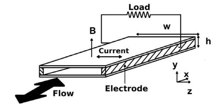
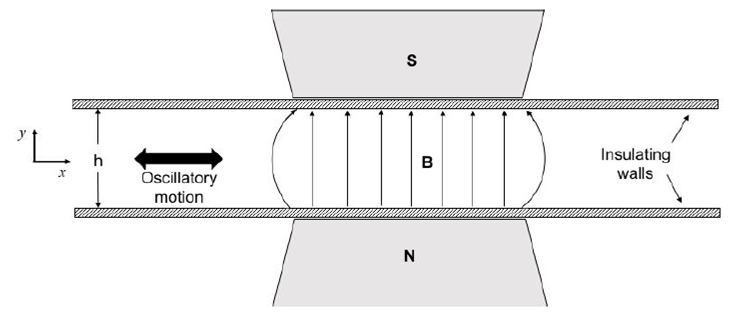
We consider the oscillatory flow of a liquid metal in a duct of rectangular cross-section under a transverse magnetic field. The walls perpendicular to the applied field are electrical insulators, while those parallel to the field are perfect conductors connected to an external load (see Fig. 1). The oscillatory flow is driven by a zero mean, time-periodic pressure gradient imposed at the extremes of the duct.

FIGURE 1 Sketch of the MHD alternate generator. 

The system of equations that govern the unsteady flow of an incompressible, electrically conducting viscous fluid in the presence of a magnetic field are the continuity equation, Navier-Stokes equation, Faraday’s law of induction, Ampère’s law, Gauss’s law for the magnetic field and Ohm’s law which, respectively, can be conveniently written in the following dimensionless form

where the flow velocity \u, the pressure p, the magnetic field B, the electric field E and the current density j are normalized by Uo=G/ρω, Gh, Bo, UoBo and σUoBo, respectively. Here, G and ω are the amplitude and frequency of the imposed oscillatory pressure gradient, ρ and σ are the mass density and the electrical conductivity of the fluid, h is the distance between the walls transverse to the magnetic field, and Bo is the maximum strength of the applied field, respectively. The coordinates (x,y,z) and time t, are normalized by h and 1/ω, respectively.

Further, the dimensionless parameters Rω=ωh2/ν, R=Gh3/ρν, Ha=Bohσρν, are the frequency parameter (or oscillation Reynolds number), the amplitude parameter and the Hartmann number, respectively, where ν is the kinematic viscosity. Assuming that the physical and geometrical properties of the system remain unchanged, these dimensionless parameters express, correspondingly, the influence of the oscillation frequency, the amplitude of the pressure gradient, and the magnetic field strength. In turn, Rm=μ0σUoh is the magnetic Reynolds number that gives an estimation of the induced magnetic field compared with the applied field ^[12], where μ0 is the magnetic permeability of vacuum.

The oscillatory motion of the fluid inside the magnetic field induces an electric current density in the spanwise (z) direction. The current, in turn, interacts with the applied field originating a braking Lorentz force in the axial x-direction. Usually, in liquid metal MHD flows the low magnetic Reynolds number approximation holds, which means that the magnetic field induced by the fluid motion is much smaller than the applied field and can be neglected ^[12]. Hence, the magnetic field is uncoupled from the fluid motion and governed by the magnetostatic equations.

3. Flow in the uniform magnetic field region

We now assume that the aspect ratio of the generator is very large, that is, w/h>>1 (see Fig. 1) so that the conducting walls (electrodes) are located at distant positions z=±zo, connected to an external electrical circuit. Under this approximation, we can consider that the oscillatory flow is two-dimensional, confined between the insulating walls transverse to the magnetic field (see Fig. 2). Since the current is induced in the direction perpendicular to the plane of motion, there must exist an electric field, Ez, the value of which depends on the external electrical load. As the magnetic field remains unperturbed, Faraday’s law of induction reduces to ∇×E=0 and the electric field becomes potential. In fact, it can be shown that under the present assumptions Ez is spatially constant and it is at most a function of time ^[16].

FIGURE 2 Two-dimensional model of the flow in an MHD alternate generator. 

We now restrict to the region where the applied field is uniform so that, in dimensionless terms, B=y^. In this region the flow is fully developed, therefore, u=u(y,t)x^ and the Navier-Stokes equation reduces to

We disregard transient solutions and consider that the harmonic axial pressure gradient that drives the flow is given by the real part of -∂p/∂x=eit. Assuming that the axial velocity component and the electric field are also harmonic functions of time, u=u0(y)eit and Ez=-Keit, with K a constant known as the load factor ^[17], a solution to the Eq.(5) that satisfies the no-slip boundary conditions can be found, namely,

where λ=Ha2+iRω and Um is the dimensionless spatial average of the velocity profile in the cross-section. From this solution it is possible to establish a model of the alternate MHD generator that allows to assess the electrical performance of the device ^[17].

In the present work the attention is focused in the interplay of inertia and the braking Lorentz force. The explicit form of the velocity profile (6) is, however, not particularly insightful. In order to get a better understanding of the physical behavior of this oscillatory MHD flow, we look for asymptotic solutions in the limits Rω≪1 and Rω≫1, which correspond to the low and high frequency oscillatory motions, respectively.

3.2 High-frequency solution: Rω≫1

At high frequencies a uniform asymptotic solution for the whole domain does not exist. Therefore, matching asymptotic solutions in the core and the boundary layer has to be sought. For the core, we start from Eq.(5) and introduce the variables u=g(y)eit and Ez=-Keit, assuming that -∂p/∂x=eit. Hence, we get the equation

ig-1=1Rωd2gdy2-Ha2(g-K). (12)

We now look for a solution g(y) as an expansion in the small parameter Rω-1, namely,

g(y)=go(y)+1Rωg1(y)+O(Rω-2). (13)

Here, we assume that Ha2=γRω, where γ is a positive real number. Then in the limit Rω→∞, from Eq.(12) and (13), the first order solution in the core is go=(1+γK)/(γ+i)=(1+γK)(γ-i)/(γ2+1). Therefore, the core velocity field is

uc=(1+γK)(γ2+1)(γcost+sint)+O(Rω-2). (14)

This represents a uniform time-periodic flow that lags behind the imposed pressure gradient according to the value of γ, where the phase angle between the pressure gradient and the core velocity is θc=-arctan[1/γ]. For γ≪1, a purely hydrodynamic flow is obtained. In this case, the Lorentz force is negligible and there is a lag of -π/2 in the motion of the core with respect to the pressure gradient. In turn, if γ=1, the Lorentz force is of the same order of magnitude as the inertial acceleration, and the core flow presents a phase difference of -π/4 with respect to the pressure gradient. When γ≫1, the Lorentz force is dominant, therefore, the phase lag is negligible and the core follows the pressure gradient oscillation.

Let us now consider the boundary layer flow. We introduce the stretched variable Y=Rω1/2(1+y) in the bottom boundary layer, hence at the wall, Y=0 and u(0,t)=0. Then Eq.(12) becomes

d2gbdY2-igb+1=γ(gb-K). (15)

for the corresponding function gb in the boundary layer. Expressing gb as a series like (13), the solution of Eq. (15) that satisfies no-slip boundary conditions and that matches with the core flow (gb∣Y≫1=(1+γK)/(γ2+1)) within an error of order O(Rω-1), leads to the boundary layer flow

u(Y,t)=(1+γK)(γ2+1)×{[γ-exp⁡(-αY)(γcos⁡βY-sin⁡βY)]cos⁡t+[1-exp⁡(-αY)(cos⁡βY+γsin⁡βY)]sin⁡t}+O(Rω-2), (16)

where

αβ=γ2+1±γ21/2, (17)

The phase angle between the boundary layer and the pressure gradient is given by

θb=arctan⁡{-[1-exp⁡(-αY)(cos⁡βY+γsin⁡βY)]γ-exp⁡(-αY)(γcos⁡βY-sin⁡βY)} (18)

Again, in-phase and out-of-phase contributions are obtained in the boundary layer, the structure of which depends on the value of γ. Provided γ≪1, a purely hydrodynamic (Stokes) boundary layer is found ^[18]. When γ=1, a mixture of Stokes and Hartmann layers results. Finally, in the case γ≫1, magnetic forces dominate and a Hartmann layer oscillating in phase with the pressure gradient (u^≈(1/Rω)[1-e-γY]cost) is obtained.

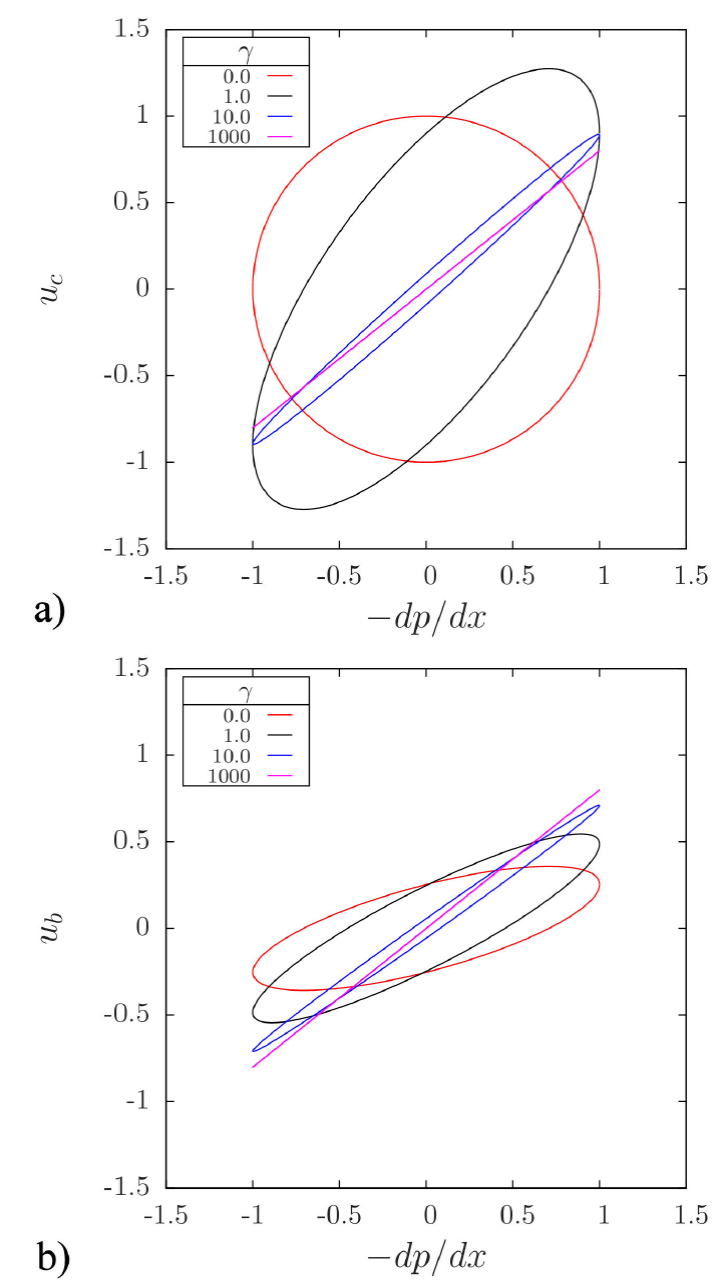
An illustrative way of visualizing the phase lag produced by the Lorentz force between the velocity and the pressure gradient is by noticing that these quantities satisfy the parametric equations of an ellipse in the plane u vs. -∂p/∂x ^[19]. If we define X=-∂p/∂x and Y=u, we get for either the core or the boundary layer flows

a2b2+1X2-2afb2XY+Y2f2b2=1, (19)

where f(γ)=(1+γK)/(γ2+1). For the core flow, a=γ and b=1, while for the boundary layer flow, we have a=γ-exp(-αY)(αcosβY-sinβY) and b=1-exp(-αY)(cosβY+γsinβY. In Figs. 3, Eq. (19) is plotted during a whole cycle for the case Rω=30, K=0.8, and different γ values. Some interesting information can be extracted from these plots, particularly because they clearly compare the velocity amplitude before and after the pressure gradient inversion. In fact, the vertical coordinate axis indicates the precise moment at which the pressure gradient is inverted. In the second and fourth quadrants, the pressure gradient acts in favor of the fluid motion, while in the first and third quadrants it acts against the fluid motion. Figure 3a shows the curves corresponding to the core flow. As it was shown, in the laminar hydrodynamic regime (γ=0, i.e.Ha=0) the core flow presents a phase difference of -π/2 with respect to the pressure gradient when Rω≫1, and the corresponding curve is a circle. For increasing values of γ, the curve is distorted and rotated clockwise as a result of stronger magnetic interaction which changes the phase difference between the velocity and the pressure gradient. When the Lorentz force is of the same order of magnitude as the inertial acceleration (γ=1), a tilted ellipse is obtained while in the case γ≫1 (Ha→∞), no phase difference exists between the flow and the pressure gradient, therefore, the curve reduces to a straight line. The corresponding curves for the boundary layer flow are shown in Fig. 3b. Although similar ellipses are formed, note that they are not the same as in the core flow since, in addition to the magnetic interaction, viscosity also affects the phase difference between the velocity and the pressure gradient. In fact, no circle is formed even when Ha=0. However, when γ≫1 (Ha→∞) a straight line is formed indicating that the phase difference disappears.

FIGURE 3 (a): The phase-like plane for the core velocity solution for different ° values and K = 0:8. (b): The phase-like plane for the boundary layer velocity solution for different ° values, Y = 0:5 and K = 0:8. 

4. Flow in the non-uniform magnetic field region

In this section, we address the oscillatory flow of the liquid metal close to the edges of the magnets where the magnetic field is non-uniform. In this region, the transverse magnetic field varies from its maximum strength to zero as the x distance to the edge of the magnet increases. Although the cross-section of the duct does not change, this can be considered as an entrance flow problem due the non-homogeneity of the magnetic field. Forced oscillations produced by the imposed pressure gradient in the outer flow produce an oscillatory flow in the Stokes-Hartmann boundary layer, however, due to the action of viscosity, the flow oscillations in this layer do not average to zero but a net steady flow is produced, known as steady streaming ^[21,^22]. The steady streaming is induced by the non-linear Reynolds stresses in the boundary layer that appear due to the axial dependence of the streamwise velocity, produced in this case by the existence of the non-uniform field. In hydrodynamic flows, steady streaming appears, for instance, at the entrance of a rigid tube when a zero-mean oscillatory flow is imposed ^[23] or in the classic problem of oscillating bluff bodies ^[22,^24]. The persistence of the steady streaming beyond the boundary layer is one of the distinctive aspects of this class of oscillatory flows ^[25]. The action of a uniform transverse magnetic field on the steady streaming produced by an oscillatory laminar boundary layer close to an insulating curved wall was previously studied using a perturbation expansion taking the inverse of the Strouhal number as a small parameter ^[26]. Following a similar procedure, we explore here the appearance of steady streaming in the boundary layers of the MHD generator promoted by the non-uniformity of the applied transverse magnetic field.

As in Sec. 3, we consider the oscillatory motion of the liquid metal limited by two infinite insulating plane walls at rest under a transverse magnetic field. We are now focused on the region close to the edges of the magnets, so the transverse magnetic field is expressed in the form B=By(x)y^ , where the variation of the field in the axial direction is given in dimensionless form as ^[15,^27]

Here x0 is a positive constant whose magnitude governs the magnetic field gradient. Figure 4 shows the magnetic field distribution for different vales of x0. We can observe that By→0 as x→-∞ and By→1 as x→∞. Although this field is not curl-free, it is a reasonable approximation that take into account the streamwise variation of the magnetic field ^[15,^27].

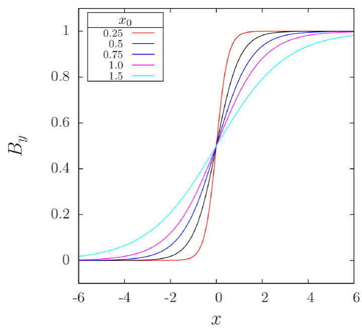
FIGURE 4 Dimensionless applied magnetic field distribution as a function of the axial coordinate x in the magnet edge region for different values of the x0 parameter. 

We assume that as a result of the imposed pressure gradient, beyond the boundary layer (outer flow) the fluid oscillates irrotationally with a zero-mean in the axial direction so that the corresponding velocity component in dimensionless form can be expressed as the real part of U(x,t)=U0(x)eit. Owing to continuity, the component of the velocity in the perpendicular direction to the wall is -(y+c)(dU/dx)eit where c is a complex constant. The governing equations of the outer flow in dimensionless form are

where the outer velocity U, the pressure p, the outer current density Jz and the electric field Ez are normalized by U∞ , σU∞B02h, σU∞B0 and U∞B0h, respectively. Here U∞ is the amplitude of the outer flow velocity. Likewise, the coordinates (x, y, z) and time t are normalized by h and 1/ω, respectively. Further, the inverse of the Strouhal number, ϵs, and the oscillation interaction parameter, Nω, ^[26] are given by

These dimensionless parameters estimate, respectively, the ratio of the amplitude of the oscillation to the characteristic length h and the ratio of the magnetic to the inertial forces. Equation (21) corresponds to the Euler equation while Equations (22) express the Ohm’s law and conservation of current in the outer flow. In order to guarantee that boundary-layer separation will not arise, the small amplitude of oscillation approximation is assumed, that is ϵs≪1.

From Eqs. (21) and (22), the explicit form of the function U0(x) can be determined at the lowest order in ϵs, namely,

where the harmonic variation of the electric field was assumed.

In turn, the inner layer flow is governed by the equations:

where U∞ and σU∞B0 have been used to normalize the velocity components in x- and y-directions (u and v) and the inner current density, jz, respectively. In order to ensure the validity of the boundary-layer approximation for the inner flow, it is assumed that Rω≫1. The boundary conditions to be satisfied by the inner flow are

where (28) and (29) represent the no-slip condition of the velocity components at the wall and (30) is the matching condition for the inner and outer flows.

4.2 Second order approximation

The equation for the second order approximation ψ1 to order ϵ has the form

∂2ψ1∂t∂y-1Rω∂3ψ1∂y3+NωBy2∂ψ1∂y=U∂U∂x-∂ψ0∂y∂2ψ0∂x∂y+∂ψ0∂x∂2ψ0∂y2. (41)

Note that the products of the harmonic functions and derivatives on the right-hand side of (41) introduce terms proportional to sin2t and cos2t, as well as steady-state terms. This means that convective non-linear terms give rise to steady state terms that contribute to the steady streaming flow. In order to solve Eq.(41) we assume that

ψ1(x,y,t)=U0dU0dxξ1t(x,y)e2it+ξ1s(x,y), (42)

where the real part of U0(x) must be taken. The equation satisfied by ξ1t is

∂3ξ1t∂y3-(Ha2By2+2iRω)∂ξ1t∂y=-Rω21-(∂ξ0∂y2+∂ξ0∂y∂2ξ0∂x∂yU0(x)U0'(x))+ξ0∂2ξ0∂y2+U0(x)U0'(x)∂ξ0∂x∂2ξ0∂y2 (43)

with boundary conditions

ξ1t(x,0)=∂ξ1t∂y(x,0)=0and∂ξ1t∂y⟶0asy⟶∞. (44)

The solution is given in the form

ξ1t(x,y)=Rω4U0'(x)κt1e-λy+κt2e-γy+κt3e-2γy+κt4 (45)

with γ=α(x)+iβ(x) and λ=αt(x)+iβt(x), where

αt(x)=Ha4By4+4Rω2+Ha2By2212,βt(x)=Ha4By4+4Rω2-Ha2By2212.

The constants κt1, κt2, κt3, and κt4 in (45) are defined in the Appendix.

Solution (45) correctly recovers the hydrodynamic solution ^[21] when the magnetic field strength tends to zero. Particularly, the contribution to the tangential velocity reduces to

∂ξ1t(x,y)∂y=12-ie-(1+i)2η+ie-(1+i)η-(i-1)ηe-(1+i)η (46)

In turn, the boundary value problem satisfied by the steady state part, ξ1s, is

∂3ξ1s∂y3-λs2∂ξ1s∂y=Rω42-2∂ξ0∂y∂ξ0∂y¯+ξ0∂2ξ0∂y2¯+ξ0¯∂2ξ0∂y2+U0(x)U0'(x)(-∂ξ0∂y∂2ξ0∂x∂y¯-∂ξ0∂y¯∂2ξ0∂x∂y+∂2ξ0∂y2∂ξ0∂x¯+∂2ξ0∂y2¯∂ξ0∂x) (47)

ξ1s=ξ1s'=0, at y=0, (48)

ξ1s'→0, as y→∞, (49)

where conjugate complex quantities are denoted by an overbar and λs=Ha2By(x). The solution of equation (47) that satisfies the required boundary conditions is

ξ1s(x,y)=RωU0'(x)κs6(κs1e-2αy+2κs2e-λsy-e-αy(κs4eiβy+κs5e-iβy)+κs3), (50)

where constants κsj(j=1 to 6) are defined in the appendix. It can be shown that taking the limit of vanishing magnetic field, Eq (50) and its derivative reduce to the corresponding expressions for the hydrodynamic flow ^[21,^26].

In the boundary layer, the second order steady velocity component parallel to the wall is given by

u1s=ϵsU0dU0dx∂ξ1s∂y,

where ∂ξ1s/∂y can be obtained from Eq.(50). In the hydrodynamic case (i.e. vanishing magnetic field) it results that, as the distance from the wall tends to infinity, u1s does not tend to zero. As a matter of fact, in this case it is not possible to satisfy simultaneously the condition u1s→0 as η→∞ as well as the non-slip condition at the wall ^[21,^25]. Therefore, the condition at infinity must be relaxed, imposing that u1s remains finite as the distance from the wall tends to infinity.

In this way, the steady streaming flow goes beyond the boundary layer, penetrating into the potential flow. The finite velocity at the edge of the boundary layer can be used as the inner boundary condition for the outer flow ^[25]. Although far form the magnet edges ∂ξ1s/∂y tends to the hydrodynamic limit as y→∞, notice that dU/dx→0 when the magnetic field is negligible. Therefore, the steady streaming disappears in the purely hydrodynamic region. Evidently, dU/dx is also zero in the uniform magnetic field region.

Unlike the hydrodynamic case, when a magnetic field is present the steady solution (50) does satisfy the vanishing of the streaming flow as the distance from the walls tends to infinity ^[26]. This means that the streaming motion does not penetrate from the boundary layer into the potential flow. Figure 5 shows the contribution to the tangential velocity ∂ξ1s/∂y as a function of the y-coordinate at a fixed position within the fringing field (x=0.5) for increasing values of Nω, with Rω=10, K=0.8 and x0=0.5. It can be observed that as Nω increases ∂ξ1s/∂y→0 and therefore the steady streaming becomes weaker as the strength of the field grows. This means that the disturbance created by streaming vortices at the extremes of the generator should not affect its performance drastically.

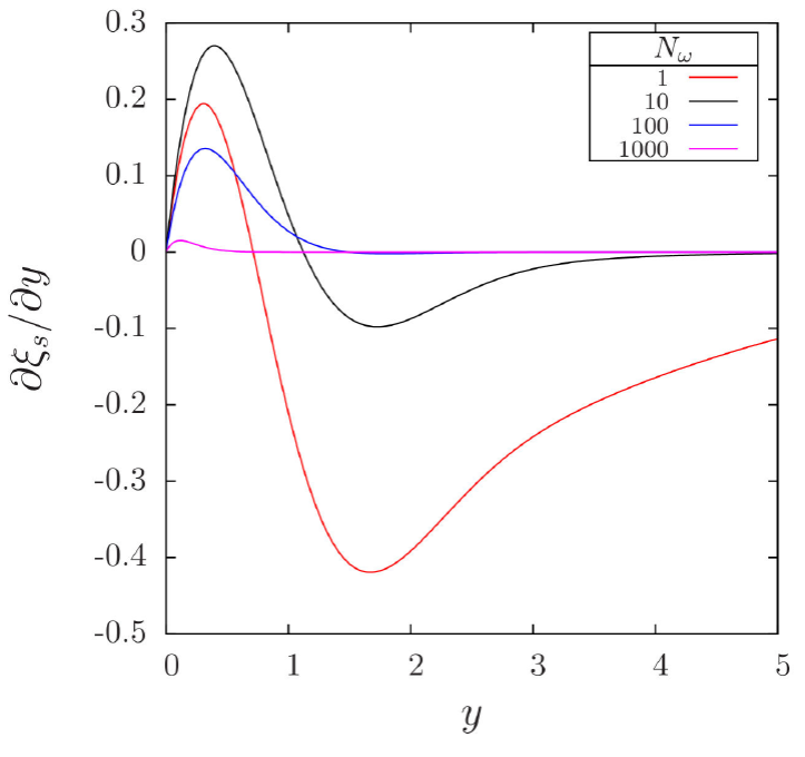
FIGURE 5  ∂ξ1s/∂y as a function of the y-coordinate for different values of N _w at a fixed position within the fringing field (x = 0:5). R _w = 10, K = 0:8 and x ₀ = 0:5. 

The steady part of the stream function, ψ1s(x,y)=U0(dU0/dx)ξ1s, is shown in Fig. 6 as a function of the x-coordinate for different values of the constant x0 that modulates the magnetic field gradient. The influence of the fringing region is clearly shown, the largest values of ψ1s occur when the field gradient is more pronounced. This shows that the stronger the magnetic field gradient the more confined the streaming vortices are and the more intense the flow is.

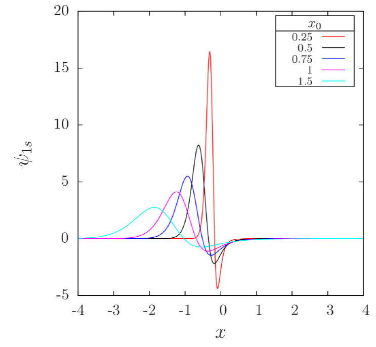
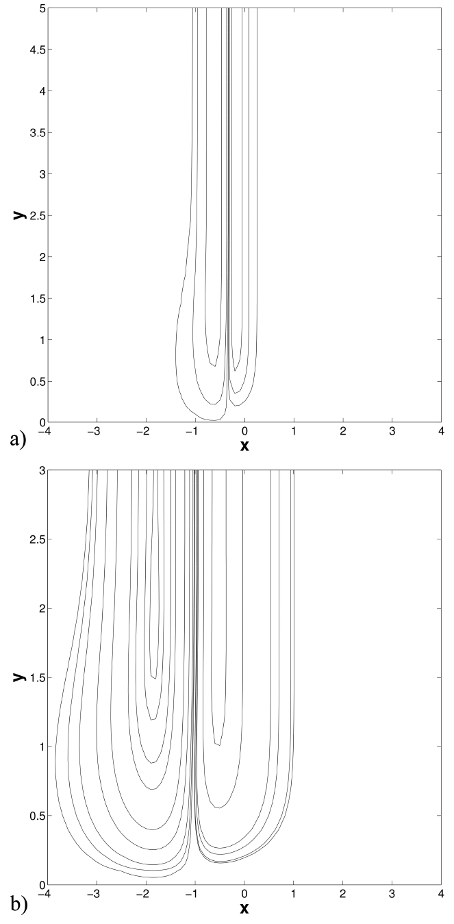
FIGURE 6 Steady part of the stream function, ψ1s(x,y)=U0(dU0/dx)ξ1s as a function of the x-coordinate at y = 1, for different values of the constant x0 that modulates the magnetic field gradient. R _w = 10, N! = 10, K = 0:8. 

In Fig. 7, the streamlines in the fringing field region are displayed for the cases x0=0.5 and x0=1.5. Two steady recirculations are observed which extend, accordingly to the value of x0, across the zone where the magnetic field passes from a uniform value to zero.

FIGURE 7 Stream lines of the steady streaming flow ψ1s(x,y)=U0(dU0/dx)ξ1s in the region of non-uniform magnetic field. R _w = 10, N _w = 10 and (a) x0 = 0:5 and (b) x0 = 1:5. 

5. Concluding remarks

We have explored the zero-mean oscillatory two-dimensional flow of a liquid metal in an alternate MHD generator driven by an imposed harmonic pressure gradient. The finite extension of the applied magnetic field transverse to the electrically insulating duct walls was considered for the analysis of the flow behavior. In the uniform field region, characteristic flows were explored through asymptotic solutions for a small (Rω≪1) and high (Rω≫1) oscillation frequencies and arbitrary Hartmann numbers. For small frequencies, a first order quasi-steady Hartmann flow in phase with the pressure gradient is obtained, while an out of phase contribution is found at O(Rω). For high frequencies a solution for the core and boundary layer was obtained. The core solution represent a uniform time periodic flow that lags from the imposed pressure gradient according to the strength of the magnetic field. When the magnetic field is negligible, a purely hydrodynamic flow is obtained and the lag between the core and the pressure gradient is -π/2. For very strong magnetic field, the lag is negligible and the core follows the pressure gradient oscillation. Out of phase and in phase contributions were also found in the boundary layer, where a purely hydrodynamic (Stokes) boundary layer is obtained for negligible field while a Hartmann layer, oscillating in phase with the pressure gradient, is obtained for strong fields. These results can be conveniently synthesized graphically.

The analysis of the entrance oscillatory flow in the fringing field region at the edges of the MHD generator was carried out for high oscillation frequencies using a perturbation method, assuming the small amplitude of oscillation approximation. From the first order solution, the thickness of the boundary layer was estimated, and it resulted a combination of the Stokes and Hartmann layers, each of which are recovered in the corresponding limits. The second order solution revealed that, superimposed to the primary oscillatory flow, a secondary flow composed by a time periodic motion oscillating with twice the original frequency and a steady streaming contribution exist. A pair of steady streaming vortices emerges in the fringing field region as a consequence of non-linear effects caused by the spatial variation of the magnetic field. The extension and intensity of the vortices grow as the magnetic field gradient increases. Unlike the hydrodynamic case, these vortices do not penetrate into the potential flow but remain confined in the boundary layer and, moreover, their strength decreases as the magnetic field becomes stronger. Although the disturbance created by the steady streaming vortices is not expected to affect the performance of the MHD generator, one could conveniently consider a smooth magnetic field gradient for design purposes.