


 text new page (beta)
 English (pdf)
 Article in xml format
 Article references
 Send this article by e-mail
 Cited by SciELO
  Similars in
SciELO
Similars in
SciELO 
 Permalink
1. Introduction
The pore systems in a sandstone could be one of four basic porosity types 1, namely: (1) intergranular, (2) porosity, (3) dissolution, and (4) fracture. In the first case, intergranular exists as space between detrital grains. In the second case, porosity exists as small pores (less than 2 μm) commonly associated with detrital and authigenic clay minerals. In the third case, dissolution is the pore space formed from the partial to complete dissolution of framework grains and/or cements. Finally, in the fourth case, fracture is the void space associated with natural fractures.
Natural gas is a gaseous mixture containing at least 75 vol.% of methane 2, and initially occupies between 30-90 % of total space of pores in the sandstone in a fresh reservoir. As an example, natural gas initially occupies between 45-60 % of pores volume at the Burgos province at the north of Mexico. Part of the volume is initially occupied by the gas and the rest of the volume is occupied by water at the bottom of reservoir. However, the reservoir is invaded by aquifer water with the gas production on the well. At the end of the productive live of the gas well, Residual Trapped Gas Saturation (RTGS) measure is a key factor to evaluate the additonal gas recovery from a drained gas reservoir, however, the measurements of RTGS exhibit values which are scattered from 5 % to 85 %. This fact represents one of the main uncertainties in the recoverable reserves of the field. To understand the measurements of RTGS some hypotheses are laid out to explain this phenomenon 3, 4. One of them is that during the gas production, water invades into the gas-saturated zone trapping a certain amount of gas independently of pores structure of the sandstone 3. Another hypothesis is that RTGS must decrease for sandstones with high porosity but it is not clear at all because for another sandstones (with similar porosity as the first one), the RTGS increases 4. At this point, the last comment suggests that the pores structure of the sandstone is the key to understand the measure of the RTGS, because at molecular level, the pores size distribution affects the displacement of methane molecules trapped into the intergranular pores or micropores 5, 6. Thus, dynamic properties (for example, the time dependent self-diffusion coefficient of methane molecules) must tell us something about the molecular confinement. In the literature, few manuscripts are focused on the self-diffusion coefficient 7-10 where the diameter of the pores is in the range of 100-500 Å. In this work, the self-diffusion coefficient is analyzed in the case of a confined gas in intergranular pores where their diameter is less or around of 20 Å. This is the goal of the present work.
The paper is divided into three main sections. Section 1 is focused on the construction of the model of the porous material and its characterization through the intergranular pores size distribution. Section 2 is focused on the analysis of the self-diffusion coefficient of the methane molecule confined into the intergranular pores of the porous material of previous section. Finally, conclusions are in the last section.
2. Model of a porous material
In this work, we focused only on intergranular porosity of a material. A micropore size definition, as the pore whose diameter is less than
A porous material is modeled as a mixture of hard spheres. In particular, the pore size distribution is analyzed. All models have the same value for the volume fraction occupied by spheres, namely,
Four models are constructed from a binary mixture of hard spheres and their configuration of species are in Table I. In the same way, another four models are constructed from a ternary mixture of hard spheres, and their specifications are in Table II. The pore size distribution is a function of the configuration of species in the mixture of hard spheres, but we can not speak about it without a previous definition of a pore, i.e. what is a pore? Moreover, if a reasonable definition of a pore is established, then what is its volume? The answer for both questions are in the following section.
TABLE I Configuration of a binary mixture of hard spheres for the model of a porous material. The value of σ0 = 18:65 °A is used as a unit length.
| Specie 1 | Specie 2 | |||
|---|---|---|---|---|
| Model | σ1/ σ0 | N 1 | σ2/ σ0 | N 2 |
| A | 1.000 | 500 | 0.100 | 1000 |
| B | 0.780 | 500 | 0.320 | 1000 |
| C | 0.550 | 500 | 0.550 | 1000 |
| D | 0.278 | 500 | 0.822 | 1000 |
TABLE II Configuration of a ternary mixture of hard spheres for the model of a porous material. The value of σ0 = 18:65 Å is used as a unit length.
| Specie 1 | Specie 2 | Specie 3 | ||||
|---|---|---|---|---|---|---|
| Model | σ1/ σ0 | N 1 | σ2/ σ0 | N 2 | σ3/ σ0 | N 3 |
| E | 1.000 | 100 | 0.500 | 900 | 0.250 | 0 |
| F | 1.000 | 100 | 0.500 | 900 | 0.250 | 500 |
| G | 1.000 | 100 | 0.500 | 900 | 0.250 | 1500 |
| H | 1.000 | 100 | 0.500 | 900 | 0.250 | 2500 |
2.1. Volume of a pore
The definition of a pore is illustrated in Fig. 1. In this case, the tetrahedron is formed by the centers of four neighbor spheres. Thus, the shape of the pore corresponds to tetrahedron volume without the partial volume of each sphere. The algorithm to calculate the pore size is now described:
1. A sphere in the matrix of hard spheres is selected (and is labeled as the sphere 1). Other three spheres, which are more close to sphere 1, are selected too. The centers of the four spheres are the corners of the tetrahedron (see the Fig. 1), and the tetrahedron volume is calculated with equation
where the vectors
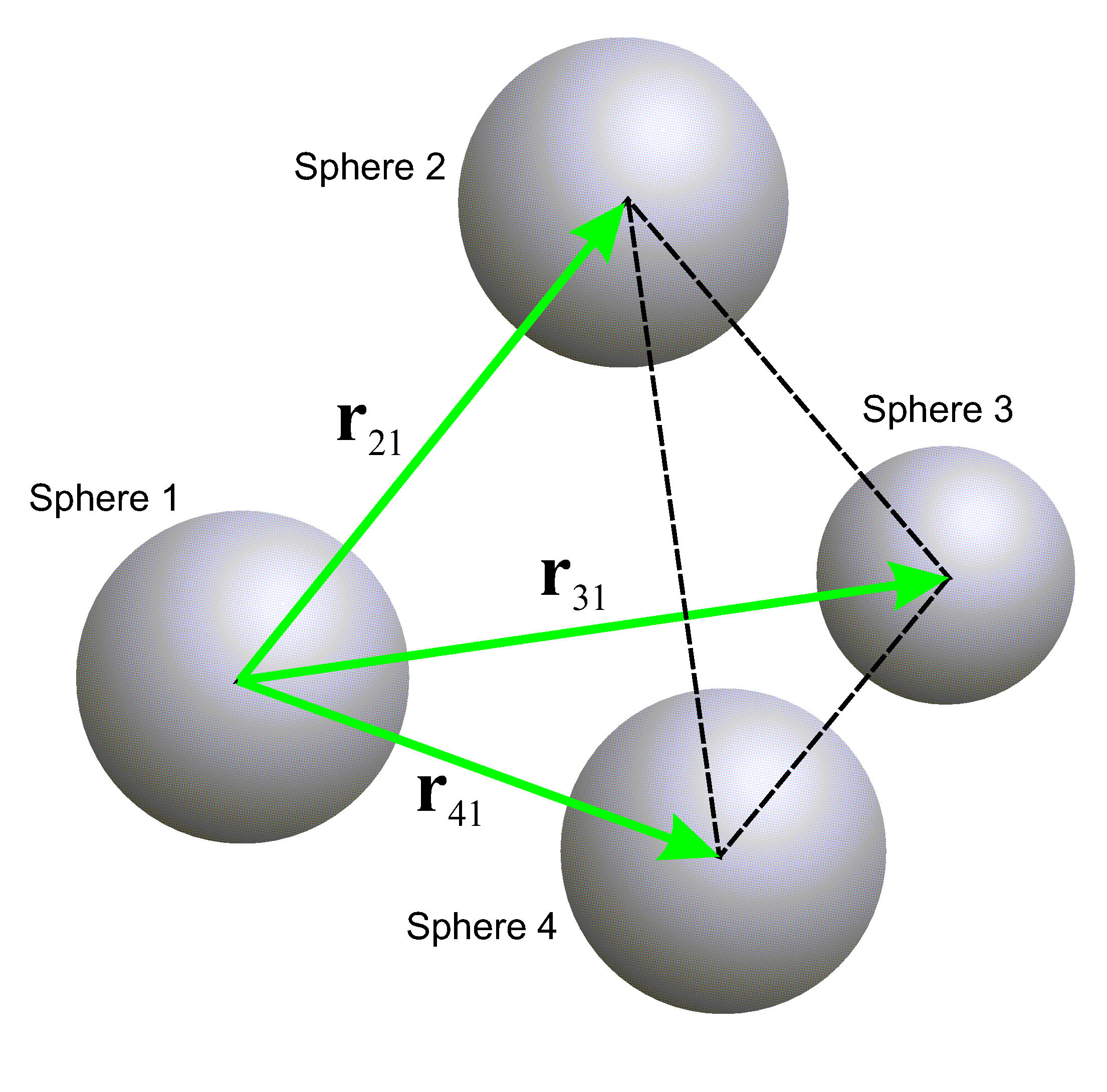
2. In this step a system of coordinate axes is chosen so that the center of the sphere

The size of the partial volume of sphere
where
3. In this final step the size of the pore is calculated with
This algorithm is applied on each sphere in the mixture of hard spheres (sandstone model) and the set of values of V will be used to construct the pore size distribution as it is described in the next section.
2.2. Pore size distribution
In order to explore different regions of the sandstone model, a set composed by
Once the construction of histogram h(V)is ended, in the next step, the histogram is normalized by using the next formula
where
In Fig. 3 the pore size distribution as a function of the pore diameter is plotted for the models A, B, C, and D reported in Table I. Model C is composed by a single specie of spheres and, in Fig. 3, its curve shows a single maximum with a narrow distribution around it. This fact tells us that the model C is characterized by a pore set of similar sizes. On the other hand, pore size distribution of models A and B show two maximums which are related to two different main sets of pores but in a narrow distribution as model C. Furthermore, the pore size distributions of models A, B, and C have a similar range of the pore size, namely,
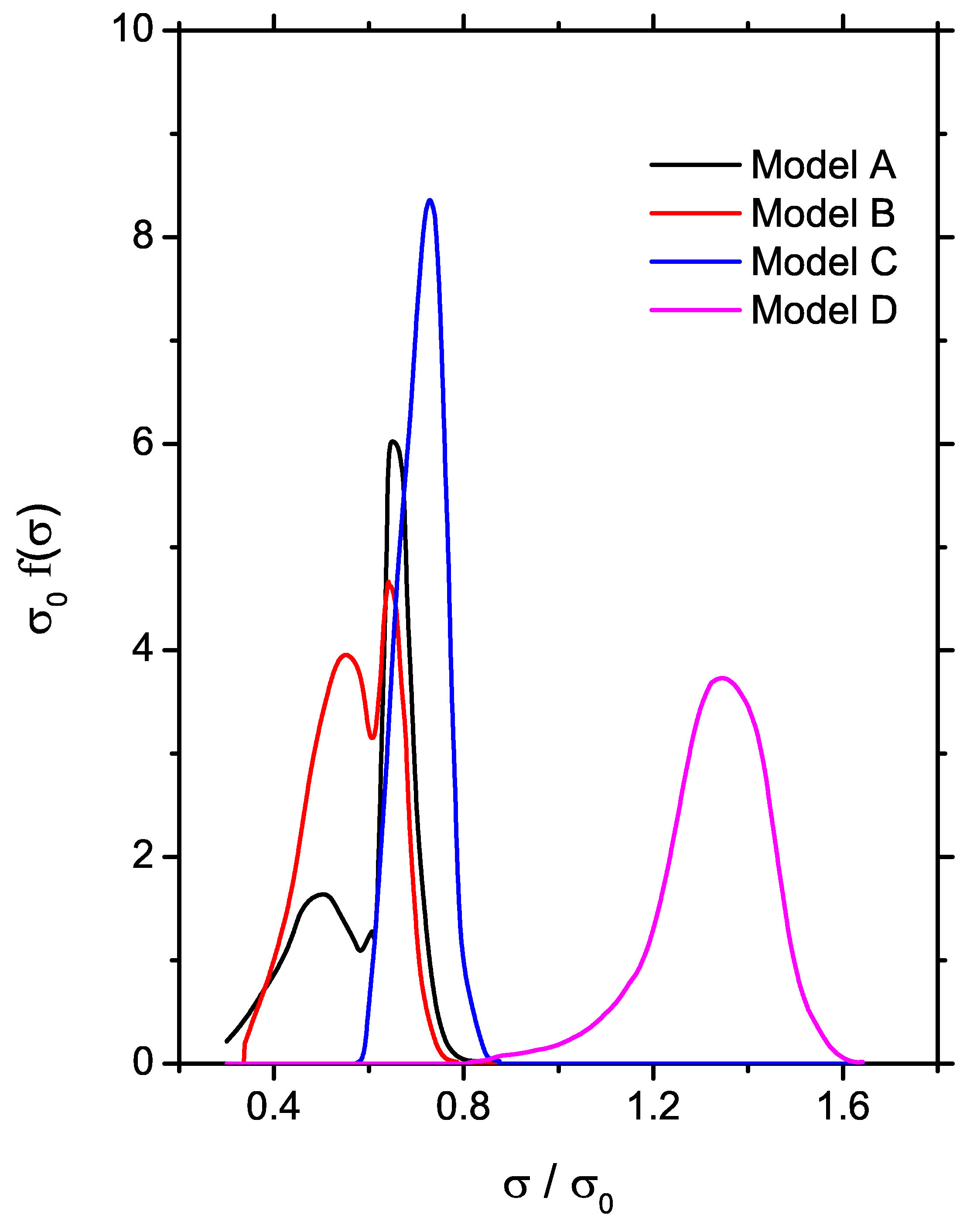
Figure 3.Pore size distribution as a function of the diameter σ of a sphere with the same pore volume. The curves correspond to the models A, B, C, and D reported in Table I.
The pore size distribution for the models E, F, G, and H (see Table II) are in Fig. 4. In these models, the number of small spheres of the third class increase from model E to model H, meanwhile the configuration of other two species does not change. Thus, the pore size decreases with the number of spheres of the third class and this fact can be to see in Fig. 4 with the shift to the left of the pore size distribution. On the other hand, model E is a binary mixture of hard spheres because the third specie is not present. In this case, the pore size distribution exhibits two maximums related to two main set of pores in the system. Models F, G, and Hare ternary mixtures of hard spheres and, in particular, the pore size distribution of models G and H is like a bell but with a soft ripple. This fact tells us that these pore size distributions have a more complex structure where, for example, model H clearly exhibits three peaks which are related to three main sets of small pores (if these pores are compared with the pore size in other models, namely,

Figure 4 Pore size distribution as a function of the diameter
Another relevant effort to characterize the porous material is by using a tracer for which its molecular displacement is affected by the temperature, the density of the fluid, and the properties of the sandstone, i.e., the pores size distribution (among other properties like the porous connectivity which is not analyzed in this work). In the next section, the model of a methane gas confined into the micropores of the sandstone is analyzed and, in particular, a dynamic property of the methane molecules will be used to characterize the system, namely, the time dependent self-diffusion coefficient of methane.
3. Sandstone and methane gas model
The construction of a sandstone model was discussed in the previous Sec. 2 and the pore size distribution was used to characterize it. At this point, the hard sphere condition for the sites of the sandstone model was only used to construct the porous material. In this section, and for the rest of the work, the hard sphere condition is removed and is substituted by a Lennard-Jones site (where its diameter is the same of previuos hard sphere). From a static matrix of sites the methane molecules (modeled with spheres) are initially placed in it in a random way. In the next step, all overlaping spheres are moved until all overlaps are completely removed. In this way, the model of a sandstone and confined gas is initially constructed. In this section, the time dependent self-diffusion coefficient of methane molecule of the gas, which is confined into the micropores of the sandstone, is discussed. The full model is illustrated in Fig. 5 where
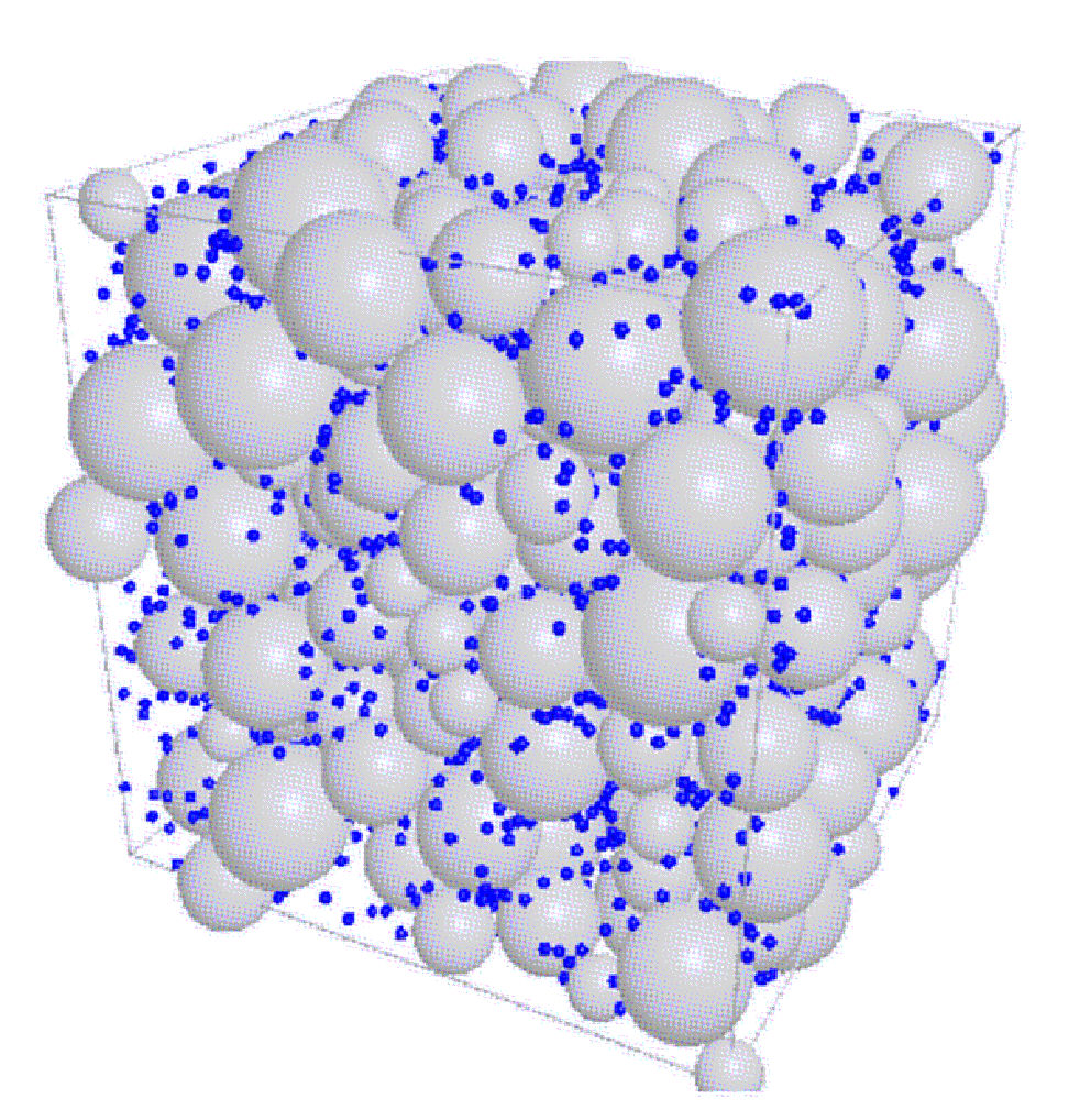
Figure 5 Illustration of the simulation box with the sandstone model (gray spheres) and the methane gas (blue spheres).
TABLE III Configuration of the sandstone and methane gas models. Ns is the number of sites in the sandstone (where, in the way, the sites are static over the time); Nm is the number of methane molecules; Vbox is the volume of the cubic simulation box; Vs = ηVbox is the volume occupied by the sites of the sandstone; Vm = xVf is the volume occupied by the methane molecules; and Vf = Vbox - Vs is the free volume available for the gas.
| Model |
|
|
|
|
|
|
|---|---|---|---|---|---|---|
| A | 1500 | 2088 | 437.2 | 262.3 | 8.7 | 174.9 |
| B | 1500 | 1125 | 235.7 | 141.4 | 4.7 | 94.3 |
| C | 1500 | 1040 | 217.8 | 130.7 | 4.4 | 87.1 |
| D | 1500 | 2359 | 494.1 | 296.4 | 9.9 | 197.6 |
| E | 1000 | 885 | 185.4 | 111.3 | 3.7 | 74.2 |
| F | 1500 | 918 | 192.3 | 115.4 | 3.8 | 76.9 |
| G | 2500 | 983 | 205.9 | 123.5 | 4.1 | 82.4 |
| H | 3500 | 1048 | 219.5 | 131.7 | 4.4 | 87.8 |
The gas molecules interact between them and with the sites of the sandstone. In particular, the total potential energy (U) is calculated and approached with the sum of the pair interactions, i.e.,
where
where the parameters are
where the parameters are
3.1. Molecular dynamics algorithm
Molecular dynamics simulation of confined gas into the porous material is performed by using the reversible in time algorithm which was proposed by Martyna 20-23. In this case, procedure to do the numerical integration of movement equations is described with the following set of equations
where
After the system is constructed with an initial valid configuration, then the molecular dynamics simulation is performed by generating at least
3.2. Self-diffusion coefficient
In this step a new molecular dynamics simulation is performed by generating a sequence of 10000 consecutive steps by using the algorithm discussed in previous Sec.3. However, the information of the dynamic state of the system is saved in a external file every
After the output file has been constructed, in the next step, the time dependent self-diffusion coefficient is calculated (from configurations which are in the output file) by using its formal definition, namely,
where
where
Self-diffusion coefficient of confined gas into the pores of a binary mixture of spheres (sandstone model) are in Fig. 6.

Figure 6 Self-diffusion coefficient of confined methane molecules into the porous material. The sandstone model corresponds to a binary mixture of spheres which its configuration is in Table I.
Curves plotted in Fig. 6 correspond to the cases A, B, C, and D which are reported in Tables I and III. Clearly, self-diffusion coefficient depends on the structure of pores as it is seen in Fig. 6. Furthermore, the sandstone models A and D have the mayor size of free volume which is available to the gas particles (see Table III), thus, self-diffusion coefficient increases apparently with the free volume. The exception is the case D. The size distribution of pores in model D (see Fig. 3) exhibits a main set of pores, meanwhile the size distribution of pores in model A exhibits two set of pores. In model
The scenario in the other sandstones, which are modeled with a ternary mixture of spheres, is also similar to the binary cases and the self-diffusion coefficient curves of the methane molecule, are plotted in Fig. 7. All the features discussed previously for the binary models of a sandstone are present in the ternary models. However, the curves in the ternary models are in general below with respect to the binary mixture cases, thus the size of pore in the ternary mixture of spheres are small with respect of the a binary mixture of spheres. Furthermore, the self-diffusion coefficient of models E, F, G, and H exhibits a high narrow peak in all curves which are plotted in Fig. 7, thus the sandstone (which is modeled with a ternary mixture of spheres) traps the gas more efficiently than the binary mixture of spheres.

Figure 7 Self-diffusion coefficient of confined methane molecules into the porous material. The sandstone model corresponds to a ternary mixture of spheres which its configuration is in Table II.
On the other hand, the initial slop of self-diffusion coefficient in all cases reported in Fig. 6 and also in Fig. 7 have the same value. To clarify this point, short-time regime 8 is defined by
where
4. Conclusions
The concentration of methane molecules is

