


 text new page (beta)
 English (pdf)
 Article in xml format
 Article references
 Send this article by e-mail
 Cited by SciELO
  Similars in
SciELO
Similars in
SciELO 
 Permalink
1. Introduction
The Riemann-Silberstein (RS) vector is defined as the complex sum of the electric and magnetic field vectors: E+ i B. It appeared in 1907 in an article by Silberstein [1], and was applied many years later by various authors to different problems [2-4] (see, in particular, Ref. [3] for a historical account and full bibliography).
The RS vector appears conspicuously in electromagnetism because it describes the electromagnetic field in a particular representation of the Lorentz group, namely an irreducible representation of the SL(2,C) group. This is evident if the method of spin coefficients is applied to the Maxwell equations.
As for the applications of spinor algebra, several formulation of the Maxwell and Einstein equations have been proposed following the pioneering article of Newman and Penrose [5]. A particulary compact formulation was worked out by Plebanski [6] in the seventies, based on the use of a null tetrad as a system of reference (see Ernst [7] for its relation with other authors formulations).
The aim of the present article is to further elucidate the role of the RS vector in the context of spinorial calculus. For this purpose, the null tetrad formalism of general relativity is used in combination with Dirac spinors, i.e. four-components spinors, and the related matrices of the Dirac algebra. The RS can thus be identified as the spinorial image of the electromagnetic field in this particular representation. Being fully covariant, our approach is valid in any Riemannian spacetime. Furthermore, it generalizes to the Maxwell equations a previous work on the Dirac equation in curved space-time [8]. The result is a particularly compact and covariant form of the Maxwell equations that can be used in combination with the Dirac equation in problems of general relativity.
2. Maxwell equations and Dirac matrices
The Dirac matrices γ α are such that
where g αβ is the metric tensor (signature {− + ++} and c = 1, in the following)
In the chiral gauge, for instance, they take the form
where σ i are the usual Pauli matrices.
Let A µ be the electromagnetic potential and f αβ = ∂ β A α − ∂ α A β the electromagnetic tensor. In flat space and Cartesian coordinates (f 01 = E x , f 12 = −B z , etc.), we have
and it follows from the definition of E = −(∂/∂t)A − ∇A 0 and B = ∇ × A in terms of A µ -which are equivalent to the homogeneous Maxwell equations-:
if the Lorentz gauge,
is used.
Accordingly, the inhomogeneous Maxwell equations take the compact form
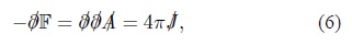
where J µ = (ρ, J) is the electromagnetic current
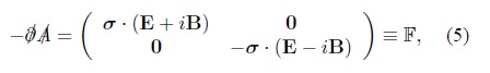
We thus see that the RS vector, defined as
appears naturally in the above representation of the electromagnetic field.
Defining
it simply follows that
The components of f µν will be identified in the context of the null-tetrad formalism (see below).
2.1. The RS vector
Defining the invariants of the field:
we have F 2 = (Ɛ + iB)2, and it follows that
Thus 𝔽2 is totally diagonal.
In the particular case of a null-electromagnetic field, Ɛ = 0 = B, the matrix 𝔽 turns out to be nilpotent of degree 2: 𝔽2 = 0.
In the general case, the matrix 𝔽 satisfies the equation
implying that the eigenvalues λ of 𝔽 are
Accordingly we have in general 4 eigenvalues, λ (i) = ±(Ɛ ± iB), with 4 eigenfunctions ψ (i) such that
Furthermore, since 𝔽2 is completely diagonal, its eigenvectors can be taken as any set of four linearly independent spinors u (i) , namely
It then follows that, in general,
which can be interpreted as a generalization to Dirac spinors of the two-components Bloch spinors (if the u (i) are chosen as constant units spinors).
3. Null tetrad formalism
The null-tetrad is a set of null-vectors
where
As shown in Ref. [8], a convenient choice of the Dirac matrices in the null-tetrad formalism is
satisfying the condition
With the above choice of Dirac matrices, it follows that in (standard) Cartesian coordinates

where the directional derivatives ∂ n are
The associated matrices σ ab = (1/2)(γ a γ b −γ b γ a ) were given in [8]; here we repeat them in the appendix for the sake of completeness. From their explicit form, it follows that for the electromagnetic tensor f ab , in particular, and for any antisymmetric tensor, f ab = −f ba , in general,
Comparing with (5), we see that the cartesian components of the RS vector F are
3.1. General coordinates system
In a general system of coordinates, the directional derivatives ∂ n must be replaced by the covariant directional derivative ∇ n . The Dirac equation in a general coordinates system can thus be written as
in terms of the covariant derivative
where Γ n are the Fock coefficients [9,10]. In a tetradial representation, they are defined as
where
with
In the null-tetrad formalism, their forms follow from (15) (see also [8]).
For a rank two tensor, in particular, we have
Applying this formula to our matrix 𝔽, one finds after some lengthy but straightforward algebra that
a formula that can also be checked by direct substitution.
Accordingly, the inhomogeneous Maxwell equations take the form
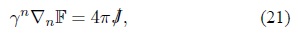
valid in general.
4. Concluding remark
The above analysis clarifies the role of the RiemannSilberstein vector in the context of a spinorial approach to classical electromagnetism. Given the full covariance of all the formulas obtained in this paper, the present formulation can be applied in future publications to problems in general relativy involving electromagnetism and Dirac fields.

