


 text new page (beta)
 English (pdf)
 Article in xml format
 Article references
 Send this article by e-mail
 Cited by SciELO
  Similars in
SciELO
Similars in
SciELO 
 Permalink
PACS: 11.10.Wx; 11.30.Rd; 12.38.Cy
1. Introduction
Among the important subjects of study in the realm of high-energy/nuclear physics, both from the theoretical and experimental points of view, are the properties of strongly interacting matter under extreme conditions of temperature and baryon density. Of particular interest is the location of the Critical End Point (CEP) in the QCD phase diagram. To this aim, the STAR BES-I program has recently analyzed collisions of heavy-nuclei in the energy range 200 GeV
Effective models have proven to be useful tools to gain insight into the phase structure of QCD. Given the dual nature of the QCD phase transition, at least for low values of
In this work we use the linear sigma model coupled to quarks, including the plasma screening effects, to explore the effective QCD phase diagram from the point of view of chiral symmetry restoration. Our strategy is to fix the coupling constants using the physical values of the model parameters, such as the vacuum pion and sigma masses, the critical temperature
2. Linear Sigma Model coupled to quarks
In order to explore the QCD phase diagram, we study the restoration of chiral symmetry using an effective model that accounts for the physics of spontaneous symmetry breaking at finite temperature and density, the Linear Sigma Model. In order to account for the fermion degrees of freedom around the phase transition, we also include quarks in this model. The Lagrangian for the linear sigma model when the two lightest quarks are included is given by
where
To allow for an spontaneous breaking of symmetry, we let the
which can later be taken as the order parameter of the theory. After this shift, the Lagrangian can be rewritten as
where
Equation (4) describes the interactions among the
respectively.
In order to determine the chiral symmetry restoration conditions as function of temperature and quark chemical potential, we study the behavior of the effective potential, which we now proceed to deduce in detail.
3. Effective potential
Chiral symmetry restoration can be identified by means of the finite temperature and density effective potential, which in turn is computed order by order. In this work we include the classical potential or tree-level contribution, the one-loop correction both for bosons and fermions and the ring diagrams contribution, which accounts for the plasma screening effects.
The tree level potential is given by
whose minimum is given by
since
which means that the curvature of the classical potential is equal to the sigma mass squared. This property is maintained even when corrections due to finite temperature and density are included in the effective potential.
However, in order to make sure that the quantum corrections at finite temperature and density maintain the general properties of the effective potential, we need to add counter-terms
These counter-terms are needed to make sure that the phase transition at the critical temperature
To include quantum corrections at finite temperature and density, we work within the imaginary-time formalism of thermal field theory. The general expression for the one-loop boson contribution can be written as
where
is the free boson propagator with
For a fermion field with mass
where
is the free fermion propagator and
The ring diagrams term is given by
where
3.1. Self-energy.
We start by computing the self-energy for one boson field. For this purpose we need to include all the contribution from the Feynman rules in Eq.(4). The diagrams representing the bosons’ self-energy are depicted in Fig. 1. Each boson has a self-energy with two kinds of terms, one corresponds to a loop made by a boson field and other one corresponding to a loop made by a fermion anti-fermion pair. Therefore, the self-energy is written as
where
with
and
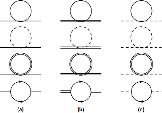
Figure 1 Feynman diagrams contributing to the one loop bosons’ self-energies. The dashed line denotes the charged pion, the continuous line is the sigma, the double line represents the neutral pion and the continuous line with arrows represents the fermions.
The leading temperature approximation to the boson self-energy is given by
This approximation, where the boson’s mass is neglected with respect to the temperature, is a good approximation around the phase transition where the boson’s mass (including its thermal correction) vanishes, namely,
On the other hand, the fermion contribution is given by
Equation (19) can be computed without resorting to assuming a hierarchy between T and
With Eqs. (18) and (20), the total self-energy for one boson is
With the boson self-energy at hand we can study the properties of the effective potential. In order to work with analytical expressions we turn to study two cases: first the high temperature approximation, i.e.
3.2. High temperature approximation
For small
Notice that Eq. (22) has two pieces, the first one is the vacuum contribution and the second one is the matter contribution, namely, the
For the case of the fermion one-loop contribution, we follow the procedure outlined for the boson case. Thus, we start by computing the sum over the Matsubara frequencies to obtain
As for the boson case, we find that Eq. (24) contains two pieces, one corresponding to the vacuum contribution and the other one to the matter contribution. The latter has the contribution of the quark chemical potential and for this reason we now have two terms corresponding to the particle and the anti-particle contributions. The vacuum contribution is computed exactly in the same manner for the boson case. For the matter term, we compute the integral in momentum taking into account the approximation where
In order to go beyond the mean field (one-loop) approximation, we need to consider the plasma screening effects. These can be accounted for by means of the ring diagrams. Since we are working in the high temperature approximation, we notice that the lowest Matsubara mode is the most dominant term24. Therefore we do not need to compute the other modes and Eq. (14) becomes
From Eq. (26), we see that both integrands are almost the same except that one is modified by the self-energy and the other one is not. Thus, after integration, we obtain that the ring diagrams contribution is
With these pieces at hand, we can write the effective potential up to the ring diagrams contribution in the high temperature approximation. This is given by
Notice that the potentially dangerous pieces coming from linear or cubic powers of the boson mass, that could become imaginary for certain values of
3.3. Low temperature approximation
To have access to the region in the QCD phase diagram where
In the case of boson fields, we include a boson chemical potential. We relate this to the energy required to add or remove one boson to the system. We associate this term to the description of high density in the analysis, in other words, the bosons’ chemical potential
In this approximation, it is not necessary to compute the vacuum and matter contributions
separately, in fact the full expression can be computed at once. In this work,
we follow the procedure used in Ref. 27.
The general idea consists on developing a Taylor series around
where
Notice that the one loop contribution from boson fields in the limit T = 0, that appears in Eq. (30), is evaluated at
For more details see Appendix C.
For fermion fields, we start from Eq. (24), such that we implement the low temperature approximation in the same way as we did for boson fields. We now develop a Taylor series around
with
Once again, we notice that the one-loop contribution from fermion fields in the limit T = 0 that appears in Eq. (33) is evaluated at
For more details see Appendix D.
Equations (6), (9), (32) and (35) provide the full expression for the effective potential in the low temperature approximation, which is given by
We are now in position to explore the QCD phase transition in the regions of the QCD phase diagram where the temperature is larger than the quark chemical potential and where the temperature is smaller than the quark chemical potential. However, before exploring the phase diagram, we need to determine the value of all the parameters involved in the linear sigma model, appropriate for the conditions of the analysis. In the following section we proceed in this direction to determine the values of those parameters and in particular of the couplings
4. Coupling Constants
Regardless of the approximation to the effective potential that is being considered, Eq. (28) or Eq. (36), we observe that we have five free parameters which should be fixed. These are the two coupling constants
We can fix a using the physical vacuum sigma and pion masses. This analysis is shown in Figs. 4-6. Alternatively, we can work in the strict chiral limit, taking
We now need to use two conditions to fix the values of the coupling constants, the main idea is to use physical inputs such that the relations which satisfy
From LQCD computations21, we know that at
In order to fix the coupling constants we use as inputs the values of temperature and quark chemical potential in two extreme points along the transition curve, namely, when the restoration of chiral symmetry is at
At point (A), the phase transition is second order, hence the square of the pion thermal mass, evaluated at v = 0 and
In other words, Eq. (38) tells us that the curvature at v = 0 and
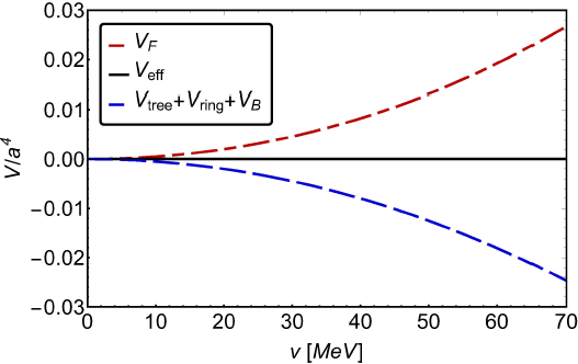
Figure 2 Fermion and boson contributions to the effective potential at the phase transition at high temperature near the minimum at v = 0. Notice that the sum of the two contributions offset each other making the potential to be flat. This is tantamount of a second order phase transition.
At point (B), the phase transition is first order, therefore we expect that at

Figure 3 Fermion and boson contributions to the effective potential at the phase transition for low temperature. Notice that the sum of the two contributions produce a barrier between each of the two degenerate minima at the transition. This is tantamount of a first order phase transition.
Since the analysis we carry out describes the transit from the broken to the restored phase, the minimum we are following is the one with a
In Eq. (39), we notice that a new unknown appears:
The three expressions in Eq. (40) indicate that the effective potential has two degenerated minima at the phase transition and thus that the transition is first order when T = 0 and the quark chemical potential is finite and equal to its critical value.
5. Results
The above set of conditions, Eqs. (38), (39) and (40), represent the five algebraic equations that determine the values of
Figures 4-6 show the phase diagram obtained for the case when the mass parameter

Figure 4 QCD phase diagram, using the physical vacuum pion mass, obtained from the solutions to the equations that deter-mine the coupling constants. These are presented in the range 0.77 < λ < 0.86 and 1.53 < g < 1.63, with µq = µb and the band’s upper line computed with
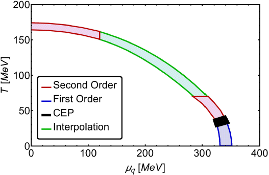
Figure 5 QCD phase diagram, using the physical vacuum pion mass, obtained from the solutions to
the equations that determine the coupling constants. These are presented
in the range 0.45 < λ < 0.49 and 1.59 < g <
1.68, with µq = 2 µb and he band’s upper line
computed with
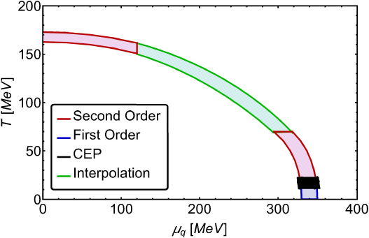
Figure 6 QCD phase diagram, using the physical vacuum pion mass, obtained from the solutions to
the equations that deter-mine the coupling constants. These are
presented in the range 0.99 < λ < 1.10 and 1.50 <
g < 1.59, with µq = 0.5µb
and the band’s upper line computed with
Figures 7-9 show the phase diagram obtained for the case when the mass parameter

Figure 7 QCD phase diagram, in the chiral limit (mπ = 0), obtained from the solutions
to the equations that determine the coupling constants. These are
presented in the range 1.02 < λ < 1.13 and 1.78 <
g < 1.89, with

Figure 8 QCD phase diagram, in the chiral limit (mπ = 0), obtained from the solutions
to the equations that determine the coupling constants. These are
presented in the range 0.58 < λ < 0.64 and 1.84 <
g < 1.96, with µq = 2µb
and he band’s upper line computed with
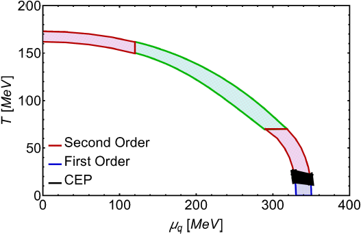
Figure 9 QCD phase diagram, in the chiral limit (mπ = 0), obtained from the solutions
to the equations that determine the coupling constants. These are
presented in the range 1.15 < λ < 1.30 and 1.74 <
g < 1.85, with µq = 0.5µb
and the band’s upper line computed with
We find that at high (low) temperature and low (high) quark chemical potential the phase transitions are second (first) order. The second order transitions are indicated by the shaded red areas and the first order transitions by the blue shaded areas. These areas represent the results directly obtained from our analysis. The intermediate green shaded area is a Padé approximation that interpolates between the high and low temperature regimes. In all cases, we locate the CEP’s region at low temperatures and high quark chemical potential.
6. Summary and conclusions
In this work we have used the linear sigma model with quarks to explore the QCD phase diagram from the point of view of chiral symmetry restoration. We have computed the finite temperature effective potential up to the contribution of the ring diagrams to account for the plasma screening effects and have introduced a quark and a boson chemical potentials. The latter is related to the high density of the system that is in turn linked to the high baryon abundance at large values of the quark chemical potential.
Our approach was to determine the model’s couplings using physical inputs such as the vacuum pion and sigma masses, the LQCD value for the critical temperature at
We find that when varying the values of
Table I Summary of some recent results for the CEP location, including our results.
| Reference | TCEP | µCEP |
| C. Shi, et al. 10 | 0.85 Tc | 1.11 Tc |
| G. A. Contrera, et al. 11 | 69.9 MeV | 319.1 MeV |
| T. Yokota, et al.30 | 5.1 MeV | 286.7 MeV |
| S. Sharma 31 | 145-155 MeV | >2 TCEP |
| J. Knaute, et al. 14 | 112 MeV | 204 MeV |
| N. G. Antoniou, et al. 15 | 119-162 MeV | 84-86 MeV |
| Z. F. Cui, et al. 12 | 38 MeV | 245 MeV |
| P. Kovács and G. Wolf 32 | >133.3 MeV | |
| R. Rougemont, et al. 16 | <130 MeV | >133.3 MeV |
| This work | 18-45 MeV | 315-349 MeV |
In order to provide a more robust CEP’s location, we need to extend the analytical expansion of the effective potential to a larger temperature range. Perhaps even more important will be to include the temperature and density modifications to the couplings which has been shown useful to describe the inverse magnetic catalysis phenomenon33. This is work for the future and will be reported elsewhere.

