Research
Research in Gravitation, Mathematical Physics and Field Theory
Recovery of transit times and frequencies of multiple pulses via the short-time Fourier transform
J. Manzanares-Martineza
C.I. Ham-Rodrigueza
B. Manzanares-Martinezb
a Departamento de Investigacion en Fisica, Universidad de Sonora, Blvd. Luis Encinas y Rosales, Hermosillo, Sonora 83000, Mexico. e-mail: jmanza@cifus.uson.mx; cavanharz@gmail.com
b Departamento de Fisica, Universidad de Sonora, Blvd. Luis Encinas y Rosales, Hermosillo, Sonora 83000, Mexico. e-mail: betsabe.manzanares@gmail.com
ABSTRACT
In this work, we present a study to determine the transit times and frequencies of pulses by using the Short-Time Fourier Transform (STFT). We consider the case of an acoustic signal composed of five Gaussian pulses that have a high overlapping in time but oscillate at different frequencies. We proceeded in three steps. First, we illustrate how the STFT calculated through a sliding window produces a spectrogram where transit time is on one axis and frequency on the other. Second, we derive an exact analytical solution of the STFT to develop an intuitive vision of the mathematical technique. Finally, in a third step, we present an experiment to demonstrate that the STFT is a useful technique to characterize a complex acoustical signal.
Keywords: Transit time; time of flight; Gaussian pulses
PACS: 43.35.+d; 43.38.+n; 43.60.+d
1. Introduction
In physics exist many pulsed signals which have a brief oscillation in time and carry a finite amount of energy. The analysis and characterization of these transient oscillations are essential for the fundamental and applied science1. The propagation of pulses is a complex phenomenon, especially if the signals are traveling through dispersive media where each frequency propagates with different phase velocity. In these systems, the pulse waveform undergoes a distortion related to the various reshaping delays as well as to the broadening and absorption.
In traditional textbooks, the transit time (τ) of a pulse is defined as the time to travel between two points2. However, when multiple pulses travel simultaneously, they interfere and produce a complicate waveform where becomes challenging to determine the transit times. One area of research where pulses are actively investigated is the transmission through waveguides. In these structures exist a discrete number of allowed frequencies. If only a mode is excited, it is relatively easy to detect the transit time by measuring between peaks. This strategy was explored experimentally by Wang et al. many years ago is the case of an elastic waveguide3. They reported the characterization of the transit time of a single pulse traveling in a thin fluid layer embedded between two elastic solids. However, some years later, Thomas et al.4. demonstrated that if multiple pulses are excited in a thicker Solid-Liquid-Solid (SLS) waveguide, the interference between them causes an undesirable deformation that makes difficult to identify the transit time by comparing the waveforms.
Recently, we have revisited this problem investigating the transit times of high-order modes
on SLS waveguides by using the Short-Time Fourier Transform (STFT)5. During this study, some of us that
did not know the STFT technique were surprised by all the information that could be
extracted of a pulse that at a first view looks only like a noisy signal5. In this work, we present a way to
understand how the STFT allows determining the transit times of multiple pulses
traveling simultaneously.
The STFT is a mathematical tool derived from the Fourier Transform. In the traditional background of Mathematical Methods in Physics, the analysis of transient signals is not a usual theme6. Some books have recently been devoted to the STFT and other related techniques as the wavelets, Gabor or Wigner-Ville. These methods are widely used by the engineering community in areas such as the digital analysis, spectral analysis, speech recognition, and radars7,8. Usually in these books are studied changes of a continues signal7-11. In contrast, here we introduce the study of the STFT considering the case of transient signals.
The main idea of the STFT is to produce a spectrogram where the transit time is on one axis and the frequency on the other9. In 1998, W. C. Lang and K. Forinash published a work on spectrograms where in their abstract presented an valuable observation:12 “While this technique is commonly used in the engineering community for signal analysis, the physics community has, in our opinion, remained relatively unaware of this development. Indeed, some find the very notion of frequency as a function of time troublesome.” After 20 years, the situation is different. Nowadays exist a broad applicability of spectrograms to analyze signals that change in time. For example, in areas such as gravitational waves13, radio astronomy14,15, nuclear dynamics16,17, or sensing of cancerous cells18.
Nonetheless, while these techniques are widely used in various areas of physics research, they are not so widely taught. In the context of the literature of physics, we have found only a few papers presenting an introductory analysis of the use of spectrograms12,19. In this work, we propose a theoretical treatment of the STFT where it is possible to obtain an analytical formula for the case of a Gaussian function. We demonstrate that this technique allows the characterization of a complex signal composed by the superposition of five pulses strongly overlapping in time. To test in the laboratory our analysis, we present an experiment where the transit time and frequency of each one of the components of a complex signal can be identified in a spectrogram.
The rest of the paper is organized as follows. In Sec. 2, we propose a succinct introduction to the STFT. In Sec. 3, we present a theoretical analysis for Gaussian pulses. In Sec. 4, is shown an experiment that demonstrates the utility of spectrograms. Finally, in Sec. 5 we have the conclusions.
2. What is the Short-Time Fourier Transform?
An example that illustrates the importance of the analysis of transient signals is the detection of the Gravitational Waves that recently proved the existence of a Binary Black Hole14. In Fig. 1 (a) we present a transient signal s(t) that is similar to the waveform received at the Laser Interferometer Gravitational-Wave Observatory (LIGO)14,15 . It is observed that in the interval Δτa there are fewer oscillations than in the interval Δτb, which means that the frequencies in these ranges are different. How can these frequencies be measured?
The analysis of frequencies based on the Fourier Transform defined by the relation
s(ω)=12π∫-∞+∞s(t)eiωtdt
(1)
is beyond reproach. However, it is not appropriate to characterize the transient signal s(t). The Fourier Transform is designed to detect the frequency components of the signal s(t) for an infinite temporal domain but does not allow to identify the localfrequencies. Additionally, the Fourier Transform cannot to determine the time-of-flight. As consequence, it is convenient to introduce a variation of the Fourier Transform to analyze transient signals.
The basic idea of the STFT is to slice the signal through a temporal window and then to determine the frequencies contained in each segment. For this reason, we introduce a window that glides performing time-localized Fourier Transforms. To illustrate how the spectrum changes over time, we introduce a function h(t-τ) that defines a temporal window centered around the time τ and zero-valued elsewhere. It is convenient to introduce the normalization of this equation as
1=∫-∞+∞h(t-τ)dτ.
(2)
In Fig. 1 (b) we present two examples of the window function h(t-τ). Using a dashed [dotted] line, we present the window functions h(t-τa) [h(t-τb)] centered at τa
[tb]. In Fig. 1 (c) are presented two transient signals that represent the function s(t) viewed through each window. The role of the window function is to isolate a temporal segment where it is possible to identify the local frequencies. To obtain a time-frequency spectrogram, we multiply the Eqs. (1) and (2) to obtain
s(ω)=12π∫-∞+∞dτS(ω,τ),
(3)
where is defined the STFT as the function
S(ω,τ)=∫-∞+∞h(t-τ)s(t)eiωtdt.
(4)
This integral can be understood as follows. The function h(t-τ) is a sliding window centered at τ which glides along the time to define local Fourier Transforms. In this manner, the STFT decomposes a time domain signal into a two-dimensional representation, where the frequency content of the transient signal is revealed inside the temporal window. Usually this integral is solved numerically, in some cases using sophisticated numerical algorithms11. To have an intuitive insight of the STFT, in the next section we present an analytical solution for a Gaussian pulse.
3. Theory
We consider an acoustic pulse in the form
pix,t=exp{-12σi2x,xi-ct]2
×cos[kix-xi-wit
(5)
The subscript i allows identifying the pulse and its components. The pulse is a solution of the acoustical wave equation, and it is composed of two functions, a Gaussian and other sinusoidal. The width of the Gaussian component is defined by σi and xi is a spatial displacement. The wave vector (ki) and the angular frequency (ωi) are related by ki=ωi/c, where c=343 m/s is the speed of sound.
3.1. A single pulse
In Figs. 2(a) and 2(b) we present the acoustic pulse for the time-dependent amplitude at the spatial points x = 0 and x = d, respectively. The parameters for the case i = 1 are σ1=0.1
m, x1=0 and f1=2
kHz. We observe that for a single pulse, it is possible to determine the transit time τ as the interval between peaks. Alternatively, the transit time can be found using the relation
Pi(x,f,τ)=∫-∞∞pi(x,t)h(t-τ)ei2πftdt.
(6)
The choice of the function h(t-τ) is an important decision because this window affects the spectral estimation of frequencies. There are different choices of windows functions as the triangular, Hann, Hamming or Gaussian.20,21 In this work, we choose a Gaussian window in the form
h(t-τ)=1τh2πexp-12τh2(t-τ)2,
(7)
where τh defines a temporal width. The integral defined by Eq. (6) can be solved analytically
and the procedure is described in Appendix
A. The solution of the integral is
Pix,f,τ=12βiτh exp{+ikix-xi-δi2
+12βi2γi+i2πf-fi]2
+12βiτh exp{-ikix-xi-δi2
+12βi2γi+i2πf+fi]2.
(8)
The functions βi2, γi and δi are defined in Appendix A. In Fig. 3 (c) we show the absolute value |P1(d,f,τ)|2 considering τh=4x10⁻⁴ s. The spectrogram in the plane (f,τ) determine the transit times and frequencies at the position x = d.
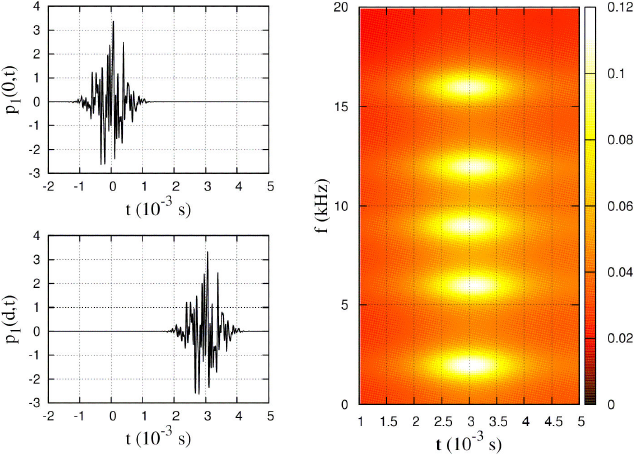
3.2. Multiple pulses
In this section we analyze a transient signal composed of the superposition of five pulses in the form
pt(x,t)=∑i=2i=6pi(x,t).
(9)
In Figs. 3(a) and 3(b) we show the pulse pt(x,t) at the points x = 0 and x = d, respectively. The parameters of are as follows. The pulse widths are σ2=σ3=σ4=σ5=σ6=0.1372 m. The phase factors are x2=0, x3=-0.01715 m, x4=+0.01715 m, x5=-0.01715 m and x6=+0.01715 m. The frequencies are f2=2 kHz, f3=6 kHz, f4=9 kHz, f5=12 kHz and f6=16 kHz. We have chosen these parameters to have pulses with a strong superposition in time. The pulse pt(x,t) has an interference pattern that looks like a noisy signal. It is evident that becomes impossible an identification of transit times comparing waveforms. However, for this kind of transient signals the STFT is a very useful tool. For this case, the spectrogram can be obtained analytically using
Pt(x,f,τ)=∑i=2i=6Pi(x,f,τ),
(10)
In Fig. 3 (c) we shown the function |Pt(d,f,τ)|2 where we have a spectrogram where it is possible to identify the frequencies and transit times of each pulse.
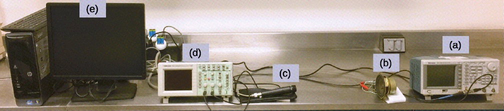
4. Experiment
The acoustic transmitting and receiving experimental setup is presented in Fig. 4. We used a Tektronix AFG3021B function generator to produce a customized time-dependent voltage signal v(t) using a software provided by the manufacturer. The signal v(t) is sent simultaneously to the oscilloscope (d) and the speaker (b). The speaker emits an acoustic pulse p(t). A Shure-SM57 unidirectional dynamic microphone placed at a distance d=0.40 m from the speaker receives an acoustical signal p'(t). The microphone produces an electrical signal that is sent to a Tektronik TDS2012 oscilloscope (d) that digitize the signal and send the information to a personal computer (e).
The transient voltage signal is defined as follows
v(t)=∑j=1j=5exp-12σj'2(x'j-ct)2cos(k'jxj-ω'jt)
(11)
The parameters are as follows, σ'1=σ'2=σ'3=σ'4=σ'5=0.343 m. We also define x1=0, x2=-0.0175 m, x3=+0.0175 m, x4=-0.0175 m and x5=+0.0175 m. The frequencies are f1=2 kHz, f2=4 kHz, f3=6 kHz, f4=8 kHz and f5=10 kHz. The wave vectors are defined by the relation kj=ωj/c.
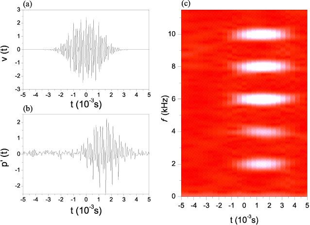
Figure 5 (a) presents the voltage pulse v(t) that is submitted from the signal generator (a) into the speaker (b). In Fig. 5 (b) we present the acoustical signal p'(t) measured by the microphone (d). We observe that it exist a complicate interference pattern that is result of the speaker signal but also exist an additional noisy contribution from the environment. In panel 5(c) we present the short time-Fourier transform of the signal p'(t) which is obtained by using the Origin software. We observe that the STFT is able to identify the transit time and frequencies of the five pulses components.
5. Conclusions
In this work, we demonstrate that the transit times and frequencies of a transient signal with a complex waveform can be recovered by using the STFT. The characterization is made using a spectrogram where the transit time is on one axis and the frequency on the other. This method of analysis has been applied to study Gaussian pulses with a sinusoidal component. For the case of a single pulse, we have found closed formulas for the STFT that allow understanding how this technique works. In the case of a pulsed signal formed by the superposition of multiple pulses, we have demonstrated theoretically and experimentally that it is possible to identify the transit times and frequencies for each pulse component.
The analysis of transient signals permits the study of many physical phenomena that can not be understood using the traditional Fourier theory. In our mathematical methods for physics, most of the work is devoted to the stationary case and the case of transient signals is rarely considered. However, as the measurement techniques have been improved, nowadays are explored a vast number of ultrafast phenomena. These signals are very important in various branches of physics, as for example the interaction of waves with nano-structures, nonequilibrium process , transient process in networks, seismological vibrations or the finding of black holes.
REFERENCES
1. S. Nolte and F. Schrempel, Ultrashort Pulse Laser Technology:Laser Sources and Applications (Springer, New York, 2017).
[ Links ]
2. L. Brillouin, Wave Propagation and Group Velocity (Academic, New York, 1960).
[ Links ]
3. W.C. Wang, P. Staecker, and R.C.M. Li, Applied Physics Letters 16 (1970) 291.
[ Links ]
4. G. Thomas, G. Komoriya, and J.P. Parekh, Journal of Applied Physics 47 (1976) 3864.
[ Links ]
5. C.I. Ham-Rodriguez, J. Manzanares-Martinez, D. Moctezuma-Enriquez, and B. Manzanares-Martinez, Applied Physics Letters 109 (2016) 061904.
[ Links ]
6. G.B. Arfken and H.J. Weber, Mathematical Methods for Physicists (Academic Press, New York, 2005).
[ Links ]
7. K.M.M. Prabhu, Window Functions and Their Applications in Signal Processings (CRC Press, New York, 2013).
[ Links ]
8. M.H. Farouk, Application of Wavelets in Speech Processing (Springer, New York, 2013).
[ Links ]
9. A. Cohen, Numerical Analysis of Wavelet Methods (Elsevier, Amsterdam, 2003).
[ Links ]
10. L. Cohen, Time-Frequency analysis (Prentice Hall, New York, 1995).
[ Links ]
11. B. Boashash, Time Frequency Signal Analysis and Processing (Elsevier, Amsterdam, 2003).
[ Links ]
12. W.C. Lang and K. Forinash, American Journal of Physics 66 (1998) 794.
[ Links ]
13. K.S. Tai, S.T. McWilliams, and F. Pretorius, Phys. Rev. D 90 (2014) 103001.
[ Links ]
14. B.P. Abbott, et al. Phys. Rev. Lett. 116 (2016) 061102.
[ Links ]
15. H. Mathur, K. Brown, and A. Lowenstein, American Journal of Physics 85 (2017) 676.
[ Links ]
16. D.A. Telnov, J. Heslar, and S.-I. Chu, Phys. Rev. A 90 (2014) 063412.
[ Links ]
17. H. Yuan, R. Zeier, N. Pomplun, S.J. Glaser, and N. Khaneja, Phys. Rev. A 92 (2015) 053414.
[ Links ]
18. D. Das et al., Phys. Rev. E 92 (2015) 062702.
[ Links ]
19. K. Meykens, B. V. Rompaey, and H. Janssen, American Journal of Physics 67, 400 (1999).
[ Links ]
20. F.J. Harris, Proceedings of the IEEE 66 (1978) 51.
[ Links ]
21. A. Nuttall, IEEE Transactions on Acoustics, Speech, and Signal Processing 29 (1981) 84.
[ Links ]
Appendix
A.
The integral of Eq. (6) can be written in the form
Pi(x,ω,τ)=122πτh∫-∞∞eα++eα-dt
(A.1)
where
α±=-12σi2 [x-xi-ct]2±i[kix-xi-ωit]
-12τh2(t-τ)2+iωt
(A.2)
Taking the squares in the first and second terms in the right side we obtain
α±=-12{βit-1βiγi+iω∓ωi}2
±ikix-xi-δ2+12βi2[γi+iω∓ωi]2
(A.3)
where we define the following functions:
βi2=c2σi2+1τh2,
(A.4)
γi=(x-xi)cσi2+ττh2,
(A.5)
and
δi=(x-xi)2σi2+τ2τh2
(A.6)
We can write
Pix,ω,τ=122πτh exp{+ikix-xi-δ2
+12βi2γi+iω-ωi2} ∫-∞+∞e-[u-]2dt
+122πτh exp{-ikix-xi-δ2
+12βi2γi+iω+ωi2} ∫-∞+∞e-[u+]2dt
(A.7)
where
u∓=12βit-1βi[γi+i(ω∓ωi)]
(A.8)
we identify
∫-∞∞e-[ui∓]2dt=2πβi
(A.9)


 nueva página del texto (beta)
 Inglés (pdf)
 Artículo en XML
 Referencias del artículo
 Enviar artículo por email
 Citado por SciELO
  Similares en
SciELO
Similares en
SciELO 
 Permalink