SciELO - Scientific Electronic Library Online

 
vol.64 número1Enhanced surface hydrophobicity of poly(lactic acid) by Co60 gamma ray irradiationTheoretical studies on the electron paramagnetic resonance parameters for the tetragonal VO2+ center in CaO-Al2O3-SiO2 system índice de autoresíndice de materiabúsqueda de artículos
Home Pagelista alfabética de revistas  

Servicios Personalizados

Revista

Articulo

Indicadores

Links relacionados

  • No hay artículos similaresSimilares en SciELO

Compartir


Revista mexicana de física

versión impresa ISSN 0035-001X

Rev. mex. fis. vol.64 no.1 México ene./feb. 2018


Research

Research in Gravitation, Mathematical Physics and Field Theory

Numerical solutions of the Maung-Norbury-Kahana equation with the coulomb potential in momentum space

Jiao-Kai Chena 

aSchool of Physics and Information Science, Shanxi Normal University, Linfen 041004, China. e-mail: chenjk@sxnu.edu.cn; chenjkphy@yahoo.com


Abstract

In this paper, the numerical solutions of the Maung-Norbury-Kahana equation which has the complicated form of the eigenvalues are presented. Taken as examples, the bound states e+e-, μ+μ- and μ+e- are discussed by employing the Maung-Norbury-Kahana equation with the Coulomb potential.

Keywords: MNK equation; virtual constituents; binding energy.

PACS: 11.10.St; 03.65.Ge; 02.60.Nm; 31.15.-p

1. Introduction

The Bethe-Salpeter equation 1 is based on the relativistic field theory and is an appropriate tool to deal with bound states. In comparison with the four-dimensional Bethe-Salpeter equation 2,3,4,5, the three-dimensional reductions of it are relatively easy to be handled . In Ref. 12, it was shown that there exist infinite versions of the reduced Bethe-Salpeter equation. One of them is the Maung-Norbury-Kahana (MNK) equation 8.

The MNK equation is covariant, obeys the unitarity relation and possesses a one-body limit. It is a proportionally off-mass-shell equation and is a relativistic, three-dimensional equation for bound states with two constituents. Moreover, the MNK equation gives a physically meaningful prescription of how the constituents go off-mass-shell in the intermediate states. The MNK equation allows the components of bound states to go off-mass-shell proportionally to their masses. In this paper, the MNK equation is solved numerically and is applied to discuss the equal-mass systems (positronium and true muonium) and the unequal-mass system (muonium).

The paper is organized as follows. In Sec. 2, the MNK equation is reviewed and the spinless MNK equation is derived. In Sec. 3, the spinless MNK equation is solved numerically and the discussions are presented. The conclusion is in Sec. 4.

2. Maung-Norbury-Kahana equation

In this section, the MNK equation is reviewed and the spinless MNK equation is derived. To discuss the bound states, e+e-, μ+μ- and μ+e-, the MNK equation with the Coulomb potential is needed. The logarithmic singularity in the momentum-space Coulomb potential is removed by the Landé subtraction method.

2.1. Reduction of the Bethe-Salpeter equation

The Bethe-Salpeter equation in momentum space reads 1,6

χPp=S1Fp1d4p'2π4×KP, p, p' χPp'S2F-p2 , (1)

where

p=η2p1-η1p2,P=p1+p2. (2)

In order to have a correct one-body limit in three-dimensional reduced equations, the Wrightmann-Gordon choice 13 of η1 and η2 should be applied,

η1=s+m12-m222s,η2=s-m12+m222s, (3)

where s = P 2. In Eq.(1), SiF(pi) are the full fermion propagators. We will approximate the full propagators SiF(pi) by free propagators 5

Si(pi)=ipi-mi+iϵ, (4)

where m1 and m2 are interpreted as effective masses for the fermion and antifermion.

We introduce components of the relative momentum p=p+p parallel and perpendicular to the bound-state momentum P by 11,14,15,16

P^=PM,M=P2,pl=pP^,p=p+p,p=plP^,p=p-plP^,d4p=dpld3p, (5)

where p is the longitudinal part and p is the transversepart. In the rest frame of the bound state with momentum P=(M,0),pl=p0,p=(p0,0) and p=(0,p). The projection operators can be written in covariant form

Λi±(p)=ωi±Hi(p)2ωi,Hi(p)=P^(mi-p),ωi=mi2+ϖ2,ϖ=-p2 (6)

with the properties

Λi(p)Λi±(p)=0,Λi+(p)+Λi-(p)=1,Λi±(p)Λi±(p)=Λi±(p),Hi(p)Λi±(p)=±ωiΛi±(p). (7)

In this paper the covariant instantaneous approximation is employed 14, in which the approximated kernel is independent of the change of the longitudinal component of the relative momentum,

K(P,p,p')K(p,p')=iV(p,p'). (8)

It is a good approximation for a system composed of heavy and light constituents or of two heavy constituents which can move relativistically as a whole. It will reduce to the instantaneous approximation in the rest frame of the bound state.

Introduce the notation for later convenience

ψP(p)=dpl2πχP(p),Γ(p)=d3p'(2π)3V(p,p')ψP(p'), (9)

where ψP(p) is the Salpeter wave function. Using Eqs. (4), (6), (8) and (9), the Bethe-Salpeter equation (1) becomes

χ(p)=G0(P,p)iΓ(p), (10)

where

G0(P,p)=g0P,p[Λ1+(p)(p10+ω1)+Λ1-(p)(p10-ω1)]P^P^×[Λ2+(-p)(p20-ω2)+Λ2-(-p)(p20+ω2)] (11)

and

g0(P,p)=1p12-m12+iϵ1p22-m22+iϵ. (12)

In Refs. 7 and 8, g0(P,p) is given as

g0(P,p)-2πiδ+f(ι)p12-m12+p22-m22+iϵ, (13)

where f(ι) is defined as

f(ι)=(p12-m12)1+ι2-(p22-m22)1-ι2. (14)

In the above equation, ι is the parameter describing the relative virtuality of two components in bound state. When ι=1, the constituent 1 is on-shell and constituent 2 are off-shell arbitrarily; vice versa, when ι=-1, the constituent 2 is on-shell with another constituent’s virtuality arbitrary. For the MNK equation,

ι=m1-m2m1+m2. (15)

Eq. (13) can be simplified as

g0(P,p)=-2πiδpl-pl+/Wp12-m12+p22-m22, (16)

where

W=(1-ι2)M2+2ι(1+ι)ω12-(1-ι)ω22 (17)

and

pl+=-1+ιη1-ιη2M+W/(2ι),-1+ιη1-ιη2M-W/(2ι). (18)

If constituent 1 takes positive energy as 0ι1 and constituent 2 takes positive energy as -1ι<0, pl+ should be

pl+=W-1+ιη1-ιη2M2ι,-1ι1. (19)

After integrating over pl, we have from Eq. (16)

g̃0(P,p)=-i/W(η1M+pl+)2-ω12+(η2M-pl+)2-ω22, (20)

From Eqs. (11), (16) and (20), we have

G~0(P,p)=g~0P,p[Λ1+(p)(η1M+pl++ω1)+Λ1-(p)(η1M+pl+-ω1)]P^P^×[Λ2+(-p)(η2M-pl+-ω2)+Λ2-(-p)(η2M-pl++ω2)] (21)

Using Eqs. (9), (19) and (21), Eq. (10) reduces to the MNK equation

ψP(p)=G̃0(P,p)d3p'(2π)3iV(p,p')ψP(p'). (22)

The MNK equation has been understood physically meaningful: when masses of constituents are not equal but comparable, this kind of choice of ι [Eq. (15)] promises that the heavier particle is less virtual while the lighter massive particles is further off-mass-shell. For the bound states composed of equally massive constituents, the constituents will be put equally off-mass-shell.

Assuming

η1M+pl++ω1η1M+pl+-ω1,η2M-pl++ω2η2M-pl+-ω2, (23)

we have from Eq. (22)

Wη1M+pl+2-ω12+η2M-pl+2-ω22η1M+pl++ω1η2M-pl++ω2ψPp= Λ1+p P^d3p'2π3 V p, p' × ψPp' P^Λ2--p (24)

Neglecting any reference to the spin degrees of freedom of the involved bound-state constituents, we have the spinless MNK equation from Eq. (24)

W[(η1M+pl+)2-ω12+(η2M-pl+)2-ω22](η1M+pl++ω1)(η2M-pl++ω2)ψP(p)=d3p'(2π)3V(p,p')ψP(p'), (25)

where ι is in Eq. (15). Eq. (25) describes the semirelativistic bound states composed to two spinless constituents which are virtual according to Eqs. (14) and (15). Following the approaches in Refs. 6 and 24, the spin-independent terms and spin-dependent terms can be obtained from Eq. (24).

2.2. Landé subtraction method

In this paper, the Coulomb potential is considered. The Coulomb potential reads in the momentum space

V(p,p')=-4πα(p-p')2, (26)

where α is the fine structure constant. The partial wave expansion of the spinless MNK equation (25) is expressed as

f(Mnl,p)ϕnl(p)=1(2π)30Vl(p,p')ϕnl(p')p'2dp', (27)

where n is the principal quantum number, l is the orbital angular quantum number. f (M, p) reads

f(M,p)=W(η1M+pl+)2-ω12+(η2M-pl+)2-ω22(η1M+pl++ω1)(η2M-pl++ω2). (28)

Vl(p,p') is the partial wave expanded Coulomb potential,

Vl(p,p')=-8π2αQl(z)pp',zp2+p'22p'p, (29)

where Q l (z) is the Legendre polynomial of the second kind,

Ql(z)=Pl(z)Q0(z)-wl-1(z),Q0(z)=12lnz+1z-1,wl-1(z)=m=1l1mPl-m(z)Pm-1(z). (30)

The Coulomb potential has the logarithmic singularity at point p' = p, and the singularity comes from Q 0(z).

Applying the Landé subtraction method 17,18,19,20,21 to cancel out the singularity, the singular equation (27) becomes

f(Mnl,p)ϕnl(p)=-αpππ22Pl(1)ϕnl(p)-απp0Pl(z)×Q0(z)p'[p'2ϕnlp'-Plz'Plzp2ϕnlp]dp'+απp0wl-1(z)ϕnl(p')p'dp', (31)

where z' = 1, Pl (1) = 1,. In the above calculation, we have used the identity

01p'Q0(z)dp'=π22. (32)

3. Numerical results and discussions

In this section, the spinless MNK equation with the Coulomb potential is solved numerically by employing the Gauss-Legendre quadrature rule. The positronium, muonium and true muonium are discussed.

3.1. Eigenvalue integral equation

The eigenvalue integral equation (31) can be written formally as

g(M,p)ψ(p)=0K(p,p')ψ(p')dp'. (33)

Due to the complicated form of g(M,p), Eq. (33) cannot be solved directly. Rewrite the above equation as 22

εψ(p)=-g(M̃,p)ψ(p)+0K(p,p')ψ(p')dp', (34)

where M̃ is a trial value. If M̃=M, ε will be equal to zero. The eigenvalue equation (34) can be solved by standard method.

3.2. Gauss-Legendre quadrature rule

Rewrite the subtracted integral equation (31) in the form of Eq. (34), then apply the Gauss-Legendre quadrature rule to the regular integral 21. Finally, a matrix equation can be obtained from Eq. (31) by employing the Nyström method and it can be solved easily.

At first, we map the semi-infinite interval [0,) onto some standard finite interval [a, b] which we take to be [-1,1). In this paper, we may take the rational transformation,

p=ξ1+s1-s,p'=ξ1+t1-t, (35)

where ξ is a numerical parameter providing additional control of the rate of convergence. Then we have

dp'=2ξ(1-t)2dt. (36)

The Gauss-Legendre quadrature formula for regular integral reads

-11f(x)dxi=0Nwif(xi), (37)

where

wi=2(1-xi2)P'N+1(xi)2. (38)

In Eq. (38), prime stands for the derivative.

3.3. Numerical results and discussions

By employing the methods discussed above, the spinless MNK equation [Eq. (25)] with the Coulomb potential is solved numerically and the numerical results are listed in Tables I, II and III. The input parameters are N = 180, ξ=miα where mi is the mass of the lighter constituent. For comparison of the eigenvalues obtained in this paper with the eigenvalues obtained in Ref. 17, the electron mass me = 0.51099906 MeV/c2, the muon mass mμ=105.658389MeV/c2 and fine structure constant α=1/137.0359895 are used 23.

Table I. Binding energies ϵnl=Mnl-m1-m2 (in eV) for a spinless electron-positron bound state (positronium) calculated by solving the spinless MNK equation [Eq. (31)], which are compared with the eigenvalues of the spinless Salpeter equation (SSE) and the Schrödinger equation (SCH). n is the principal quantum number, l is the orbital angular quantum number. A negative sign before the energy has been omitted everywhere. 

Table II. Same as Table I, except for a spinless muon-antimuon bound state (true muonium). 

Table III. Same as Table I, except for a spinless muon-electron bound state (muonium). 

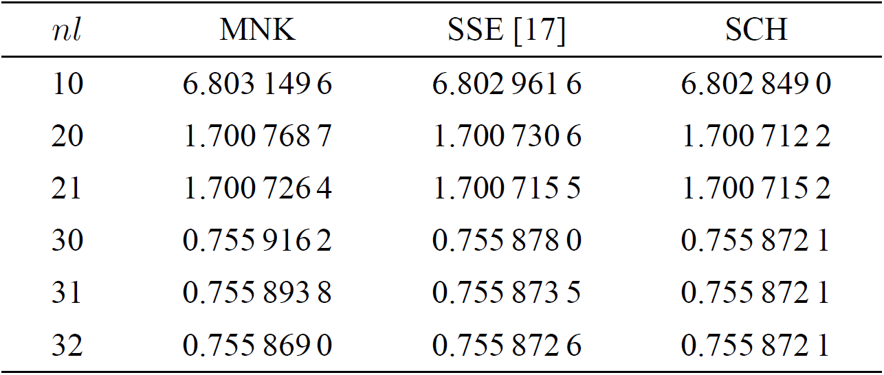
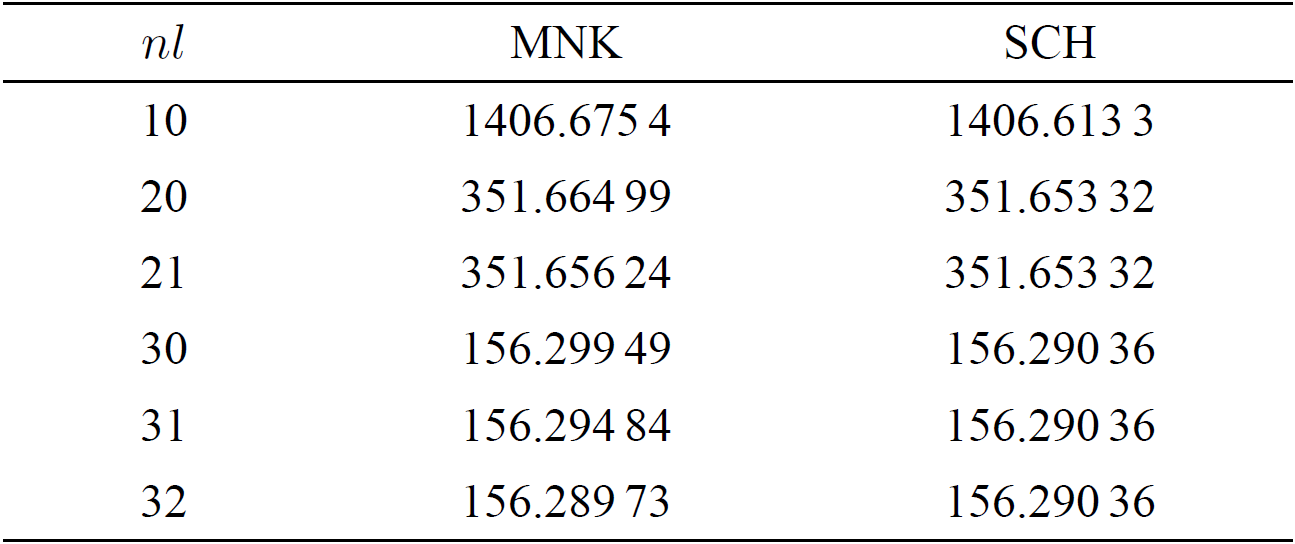
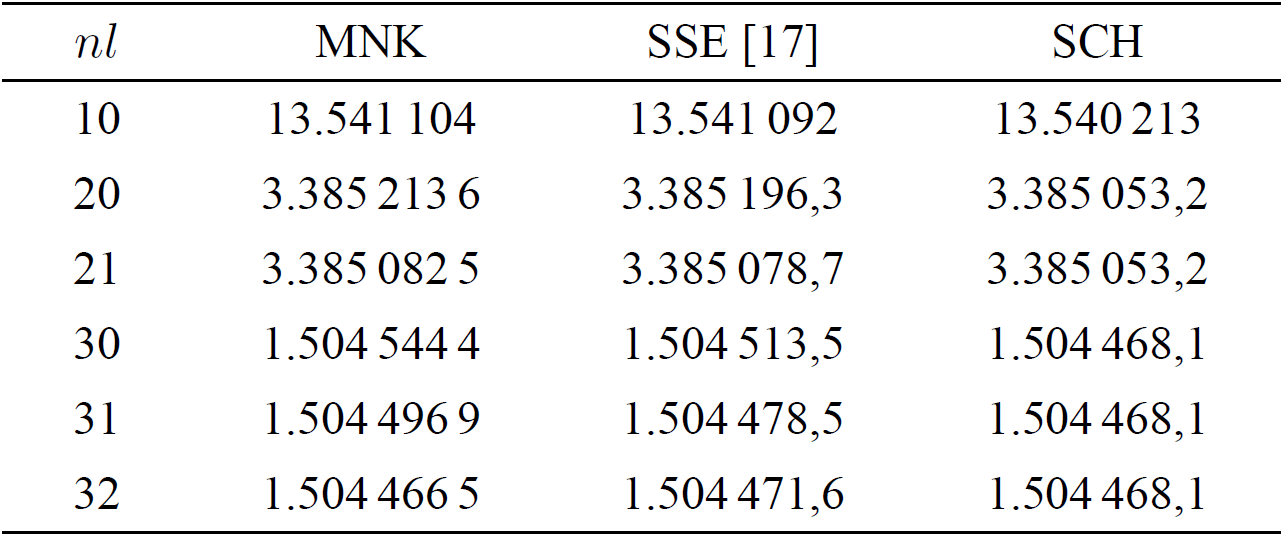
In the spinless MNK equation (25), the virtuality parameter ι is expressed in Eq. (15). As -1<ι<1, constituents are virtual. As ι=±1, regardless whether the constituents are light or heavy, the spinless MNK equation (25) reduces to the spinless Salpeter equation 17 in which both of constituents are on their mass shell. The spinless Salpeter equation is a well-defined standard approximation to the Bethe-Salpeter equation and a relativistic extension of the nonrelativistic Schrödinger equation. By comparing the binding energies of the Schrödinger equation and that of the spinless Salpeter equation, we can obtain the relativistic effects because the constituents are also put on-mass-shell in the Schrödinger equation as in the spinless Salpeter equation. From Tables I, II and III, we can see that the relativistic corrections are the differences in energies which occur after a few decimal places.

The spinless MNK equation includes not only the relativistic effects but also the virtuality effects. By comparing the eigenvalues of the spinless MNK equation and that of the spinless Salpeter equation, we can obtain the virtuality effects. The eigenvalues of the spinless MNK equation are smaller than that of the spinless Salpeter equation and the Schrödinger equation, see Tables I, II and III. It means that the virtuality effect of constituents results in stronger binding. For the positronium, the virtuality effect is about of the same order as the relativistic effects. For the muonium, the virtuality effect is smaller than the relativistic effect. The data show that the virtuality effect varies with the virtuality parameter ι. For more general cases, the relation between the virtuality effect and ι will become complex 22.

The spinless MNK equation (25) describes the bound states composed of the spinless virtual constituents. By employing the approaches applied in Refs. 6 and 24, the spin-independent terms and spin-dependent terms can be obtained from Eq. (24). Then spin effects can be included according to the discussed problems.

4. Conclusion

In this paper, the spinless Maung-Norbury-Kahana equation is derived and is solved numerically. Taken as examples, the positronium, muonium and true muonium are studied by employing the spinless MNK equation with the Coulomb potential. The MNK equation allows the constituents of bound states to go off-mass-shell proportionally to their masses. The numerical results show that the binding of virtual constituents will be stronger than that of the on-mass-shell constituents and the virtuality effect varies with different virtuality parameter ι and different mass ratio m1/m2.

Acknowledgements

We are very grateful to the anonymous referee(s) for the valuable comments and suggestions.

References

1. E.E. Salpeter and H.A. Bethe, Phys. Rev. 84 (1951) 1232; E.E. Salpeter, Phys. Rev. 87 (1952) 328. [ Links ]

2. J. Carbonell, T. Frederico and V.A. Karmanov, Eur. Phys. J.C 77 (2017) 58; J. Carbonell and V.A. Karmanov, Phys. Rev. D 90 (2014) 056002; V.A. Karmanov, J. Carbonell and M. Mangin-Brinet, Nucl. Phys. A 790 (2007) 598c; S.M. Dorkin, L.P. Kaptari, C.C. degli Atti and B. Kampfer, Few Body Syst. 49 (2011) 233. [ Links ]

3. W. de Paula, T. Frederico, G. Salmè and M. Viviani, Phys. Rev. D 94 (2016) 071901; T. Frederico, G. Salmè, M. Viviani, Phys. Rev. D 85 (2012) 036009; K. Kusaka, A.G. Williams, Phys. Rev. D 51 (1995) 7026; V.A. Karmanov, J. Carbonell, Eur. Phys. J.A 27 (2006) 1. [ Links ]

4. N. Nakanishi, Prog. Theor. Phys. Suppl. 43 (1969) 1; Prog. Theor. Phys. Suppl. 95 (1988) 1. [ Links ]

5. J. Resag, C.R. Munz, B.C. Metsch and H.R. Petry, Nucl. Phys. A 578 (1994) 397; W. Lucha and F.F. Schöberl, Phys. Rev. D 87 (2013) 016009. [ Links ]

6. J.K. Chen, Z.X. Tang and Q.D. Chen, Mod. Phys. Lett. A 22 (2007) 2979; J.K. Chen and Y. Liu, IL Nuovo Cimento B 122 (2007) 1. [ Links ]

7. F. Gross, Phys. Rev. C 26 (1982) 2203; F. Gross, Phys. Rev. 186 (1969) 1448. [ Links ]

8. K.M. Maung, J.W. Norbury, and D.E. Kahana, J. PHys. G: Nucl. Part. Phys. 22 (1996) 315. [ Links ]

9. E.D. Cooper and B.K. Jennings, Nucl. Phys. A 500 (1989) 553; V.G. Kadyshevsky, Nucl. Phys. B 6 (1968) 125; K. Erkelenz, Phys. Rept. 13 (1974) 191; R.H. Thompson, Phys. Rev. D 1 (1970) 110. [ Links ]

10. T. Kopaleishvili, Phys. Part. Nucl. 32 (2001) 560; [Fiz. Elem. Chast. Atom. Yadra 32 (2001) 1061]. [ Links ]

11. A. Klein and T.S.H. Lee, Phys. Rev. D 10 (1974) 4308. [ Links ]

12. R.J. Yaes, Phys. Rev. D 3 (1971) 3086. [ Links ]

13. A.J. MacFarlane, Rev. Mod. Phys. 34 (1962) 41; P.C. Tiemeijer and J.A. Tjon, Phys. Rev. C 49 (1994) 494. [ Links ]

14. Y.B. Dai, C.S. Huang and H.Y. Jin, Phys. Rev. D 51 (1995) 2347. [ Links ]

15. C.H. Chang and Y.Q. Chen, Commun. Theor. Phys. 23 (1995) 451; C.H. Chang, J.K. Chen and G.L. Wang, Commun. Theor. Phys. 46 (2006) 467. [ Links ]

16. J.K. Chen, Rev. Mex. Fis. 62 (2016) 235; J.K. Chen, Chin. J. Phys. 53 (2015) 100201; C. Chen and J.K. Chen, Pramana 86 (2016) 809. [ Links ]

17. J.W. Norbury, K.M. Maung, and D.E. Kahana, Phys. Rev. A 50 (1994) 3609. [ Links ]

18. R.H. Landau, Phys. Rev. C 28 (1983) 1324; R.H. Landau, Phys. Rev. C 27 (1983) 2191; Y.R. Kwon and F. Tabakin, Phys. Rev. C 18 (1978) 932. [ Links ]

19. J.W. Norbury, K.M. Maung, and D.E. Kahana, Phys. Rev. A 50 (1994) 2075. and references therein; A. Tang and J.W. Norbury, Phys. Rev. E 63 (2001) 066703; K.M. Maung, D.E. Kahana, and J.W. Norbury, Phys. Rev. D 47 (1993) 1182; J.W. Norbury, D.E. Kahana, and K.M. Maung, Can. J. Phys. 70 (1992) 86. [ Links ]

20. J.K. Chen, Phys. Rev. D 86 (2012) 036013; Phys. Rev. D 89 (2014) 099904(E); J.K. Chen, Few-Body Syst. 54 (2013) 2081. [ Links ]

21. J.K. Chen, Phys. Rev. D 88 (2013) 076006. [ Links ]

22. Jiao-Kai Chen, submitted. [ Links ]

23. L. Montanet et al. [Particle Data Group], Phys. Rev. D 50 (1994) 1173; K. Hikasa et al. [Particle Data Group], Phys. Rev. D 45 (1992) S1; Phys. Rev. D 46 (1992) 5210(E). [ Links ]

24. D. Gromes, Nucl. Phys. B 131 (1977) 80; A. Gara, B. Durand, L. Durand and L.J. Nickisch, Phys. Rev. D 40 (1989) 843; A. Gara, B. Durand and L. Durand, Phys. Rev. D 42 (1990) 1651; Phys. Rev. D 43 (1991) 2447(E). [ Links ]

Received: July 24, 2017; Accepted: September 05, 2017

Creative Commons License This is an open-access article distributed under the terms of the Creative Commons Attribution License