


 text new page (beta)
 English (pdf)
 Article in xml format
 Article references
 Send this article by e-mail
 Cited by SciELO
  Similars in
SciELO
Similars in
SciELO 
 Permalink
1. Introduction
The subject of Quantum Field Theory at finite temperature rises from the observation that non-abelian gauge theories at zero temperature are broken but that they are restored at high temperatures1. This means that in eras when some phenomena of elementary particles were relevant for the evolution of the universe, the temperature was extremely high. Then, when we apply elementary particles theory to the early universe, temperature must be taken into account2. Also at high temperatures QCD loses its confinement and thermal excitations generates a plasma of quarks and gluons screening the color electric flux3.
The radiative corrections to some physical quantities receive contributions dependent of temperature also. Several authors have calculated finite temperature radiative corrections to neutron decay4, to primordial nucleosynthesis2, and to the magnetic dipole moment of muon or electron By finite temperature we must understand “in the presence of a distribution of particles in thermal equilibrium (the thermal bath)”. These works were done in the real time method because a separation of temperature contributions is quite direct15. The characteristic feature of this formalism is the doubling of the degrees of freedom, that is, to each physical field a ghost field has to be introduced, but only the physical ones on the external legs16. The propagator assumes a 2×2 matrix structure, and for each vertex there exist now a complex conjugate ghost counterpart. The full matrix structure of the theory is necessary only in higher orders in perturbation theory: this doubling of fields ensures the cancellation of ill-defined distributions arising from self-energy insertions on internal lines in multiloop diagrams17. As is known, the real-time formalism agrees with the imaginary-time formalism in the scalar case and in the case of fermions with zero chemical potential18.
In the present paper we calculate, following Ref. 7, the radiative corrections to the magnetic moment of a charged lepton (electron, muon or tau) from the virtual photon and its supersymmetric partner, the photino, in the minimal extension of the standard model of electro-weak interactions (MSSM). The virtual exchange of susy particles can contribute to the magnetic moment of fermions. Some authors have used the experimental results at zero temperature to constraint the masses of the photino and the lepton scalar partners. A well known result in field theories with spontaneously broken symmetries is that they behave like magnets, where magnetization vanishes beyond Curie temperature, restoring rotational symmetry. However, since bosons and fermions responds differently to temperature, supersymmetry is spontaneously broken at finite temperature19, but the degree of rupture is small even at the temperature 𝑇≈ 10 15 K, when it is believed that exact supersymmetry ends. A recent analysis of the constrained supersymmetric standard model, suggests that the model is still compatible, and not ruled out, with the present experimental constraints20.
The paper is organized as follows. In Sec. 2 we present the set of Feynman rules required for the calculation, and obtain the amplitudes for the different contributions from particles and sparticles. In Sec. 3 we explicitly calculate the radiative correction from the virtual photon and photino pair, and in Sec. 4 those from the virtual lepton-slepton pair. In Sec. 5 we discuss our result in the limit of exact supersymmetry.
2. Feynman rules at finite temperature
To calculate the radiative corrections at finite temperature, we need the propagators of the photon, the fermions and of the scalars in the loop. These are taken from Ref. 7. For the photon of 4-momentum k the propagator is
where
is the photon propagator at zero temperature, and
is the Bose-Einstein distribution function. The exponent 𝛽⋅𝑘 represents the scalar product of the 4-vector 𝑘 𝜇 with the 4-vector 𝛽 𝜇 =(1/𝑘𝑇,0) in the thermal bath reference system, 𝑇 being its temperature. For fermions of mass 𝑚 and 4-momentum 𝑝, the propagator is given by
where
is the zero temperature propagator, and
is the Fermi-Dirac distribution function. For scalars of mass 𝑚 and 4-momentum 𝑘, the corresponding propagator is
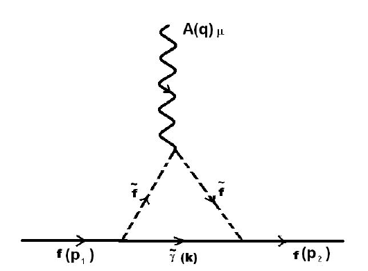
Figure 2 Feynman diagram for the photino ° contribution. The fragmented lines (labeled ef), represents the slepton partners to the external fermions.
with
the zero temperature scalar propagator.
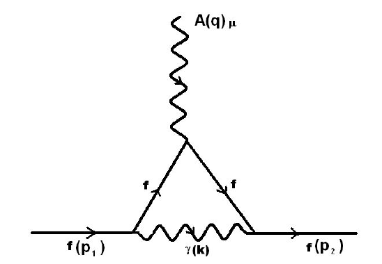
The radiative corrections we consider in this work are depicted in Figs. 1 and 2, corresponding to the virtual photon and leptons, and virtual photino and sleptons, respectively. The amplitude from Fig. 1 is given by
In (9), 𝑢( 𝑝 1 ) and 𝑢( 𝑝 2 ) are Dirac spinors for the initial and final fermions, 𝜀 𝜇 (𝑞) is the external photon polarization 4-vector, and
After substitution, from (1) and (4), of photon and fermion temperature dependent propagators in (10), we obtain
where
 (12) , (13)
Here 𝛥 𝔐 𝜇 = 𝔐 𝜇 − 𝔐 𝜇0 , with 𝔐 𝜇0 is the zero temperature amplitude.
The amplitude from Fig. 2 is
where
The parameters A and B give the scalar and pseudoscalar couplings in the lepton - slepton - photino vertex. After substitution of (4) and (7), for the photino and slepton temperature dependent propagators, we obtain
with
Here 𝑚 and 𝑚 𝛾 are the masses of the slepton and photino in the loop, respectively.
3. Radiative corrections from virtual photon and photino
The contribution (11) is the one coming from the virtual photon, while those from (12) and (13) come forth the virtual leptons in the loop. To evaluate (11), we substitute fermion propagators at zero temperature from (5),
The restriction 𝑘 2 =0, imposed by the Dirac delta, has been applied, and
where the ellipsis contains terms that do not contribute to the magnetic moment. The evaluation of (18) has been performed in Ref. 7; we rewrite the result in the form
with
and
Evaluation is easily performed in the static limit 𝑞 2 =0, giving
where 𝐷 1 =( 𝑝 2 𝑠 2 − 𝑏 2 ) 2 +4 𝑁 2 (𝛽⋅𝑝 ) 2 𝑠 2 and 𝑏=𝑁 𝛽 0 . Then,
The sum over 𝑁 gives the Spence function, defined as
After considering that $\overline{u}(p_{2}){/ \hspace{-5pt} p}u(p_{1})=2m$ 𝑢 ( 𝑝 2 )𝑢( 𝑝 1 ), we obtain
The contribution to the magnetic moment is within the square bracket,
The contribution 𝔐 𝜇 (1) is the analogous one to 𝔐 𝜇 (1). We make the same algebraic steps to get
where 𝛿 = 𝑚 2 − 𝑚 2 + 𝑚 𝛾 2 , with the terms contributing to the magnetic moment given by
and
To obtain an analytical result we proceed as follows. For the first term in (26), already proportional to the photino mass, which we denote by 𝔐 𝜇 (1 ) ′ , we neglect the contribution on the mass of the photino in the argument of the delta function, to obtain
with 𝑓( 𝑧 1 ) identical to 𝑓( 𝑧 1 ), but replacing 𝑧 1 instead of 𝑧 1 ,
and in the static limit 𝑞 2 =0, 𝑧 1 2 = 𝑝 2 𝑠 2 , 𝛽⋅ 𝑧 1 =(𝛽⋅𝑝)𝑠. The 𝑣-integral is simple, and the integral over 𝑠 is evaluated using the Mathematica program, leading to Meijer’s G-functions,
Now, substitution of (28) in (14) shows that this contribution to the magnetic moment has a factor 𝐴 2 − 𝐵 2 , which vanishes because in the MSSM the parameters A and B take the same value 𝑖𝑒/ 2 .
For the second contribution in (26), denoted by 𝔐 𝜇 (1 ) ′′ , we again assume 𝑚 𝛾 2 =0 in the delta function and take the static limit, to obtain
with 𝛤 𝜇 ( 𝑧 1 ) as in (26). The integral is evaluated using the same program and gives
where
with
We rewrite Eq.(30) as
then, its contribution to (25) is
The term in 𝛾 5 does not contribute to the magnetic moment. In the MSSM the parameters A and B take the same value 𝑖𝑒/ 2 , then 𝐴 2 + 𝐵 2 = ?? 2 . Besides, we must take into account that there are two scalar ( 𝑓 𝐿 and 𝑓 𝑅 ) in order to match the number of helicity states with those of the virtual fermions in Fig. 1. In this way we have
The term in square brackets is the contribution to the magnetic moment
4. Radiative corrections from virtual lepton and sleptons
The contribution from (12) is
 (35)
(35)
where 𝛥 𝜇 ( 𝑧 2 ) is given by the same expression as 𝛥 𝜇 ( 𝑧 1 ), but
(the contribution (13) can be obtained after the substitution 2↔1 in the indexes in (12)). The integration over the variable 𝑣 has no analytic result unless we take 𝑚 2 =0 in the exponential function, allowing for an integration over the variable
 (36)
(36)
with
The contribution to the magnetic moment is
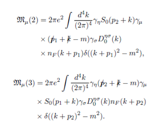
The contribution from the virtual sleptons is given by 𝔐 𝜇 (2) and 𝔐 𝜇 (3),
 (39)
(39)
where 𝛿 ′ = 𝑚 2 + 𝑚 2 − 𝑚 𝛾 2 and
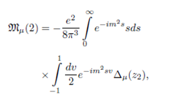
The integrals in (39) are of the same form as those in (36), and to obtain an analytic result we put 𝛿 ′ =0 in the exponential function in the integration over the variable 𝑣 , allowing for an integration over the variable 𝑠,
where
The result for the anomalous magnetic moment is
5. Conclusions
In summary, we have calculated,under some approximations, the radiative corrections to the anomalous magnetic moment of a charged lepton from virtual photon, photino, lepton and sleptons in the supersymmetric version of the standard model. The respective contributions are given by analytic functions of the temperature 𝑇 in Eqs. (24), (34), (38) and (42).
It is interesting to note that when we consider the result (34) in the limit of exact supersymmetry, i.e. when 𝑚 =𝑚 and 𝑚 𝛾 =0, and since Meijer’s functions are defined only when its argument is different from zero, it is better to take this limit before evaluation of the integral in (29). Then, the result for the magnetic moment is
Adding this result to (24) we obtain
which vanishes since 2𝐿 𝑖 2 (−1)=−𝐿 𝑖 2 (1). Then, in the limit of exact susy, the radiative correction to the magnetic moment of a charged lepton at finite temperature from the pair photon-photino, vanishes as in the case of temperature 𝑇=0 22 However this is not the case for the other contributions, as can be seen from (38) and (42). As is stressed in19 in a supersymmetric theory bosonic and fermionic contributions tend to cancel each other at 𝑇=0, but at high temperatures supersymmetry must be broken.

