


 text new page (beta)
 English (pdf)
 Article in xml format
 Article references
 Send this article by e-mail
 Cited by SciELO
  Similars in
SciELO
Similars in
SciELO 
 Permalink
PACS: 82.40.Bj; 05.45a; 02.30.Oz
1. Introduction
The Tantalus oscillator is a hydrodynamic system that behaves as a nonlinear oscillator with a stable limit cycle. Oscillators with stable limit cycles are abundant among many kinds of systems: physical 1, chemical 2 physiological 3, electronic 4,5, etc. The description of their dynamical behavior may be very complex however, their general properties under perturbations can be described recurring to the Reset Theory 6,7. The fundamental tool in this theory is a map or function called Phase Transition Curve (PTC), which describes the punctual effect of isolated perturbations given at specific moments to the particular nonlinear oscillator studied. More recently systems that are described by discontinuous maps have become relevant, for example, oscillators that suffer impacts 8,9, electric circuits 10,11, dc-dc converters 12, etc. As it has been shown in a series of theoretical studies, in these systems the discontinuity has a border role since it divides different kinds of behavior in the map 13. The discontinuity can occur directly in the function or in its derivatives 14, and it can induce the existence of Border Collision Bifurcations (BCB) which happen when a fixed point or an element in the orbit collides with the discontinuity and changes the dynamical behavior 15. Also this type of map can originate a One-parametric Bifurcation Diagrams which has a staircase shape 16. Moreover to generate points that coincide with an infinite number of bifurcations lines that have been named Big Bang Bifurcations points (BBB) 17.
The Tantalus oscillator was studied previously by Chialvo et al. in 1991 18; these authors showed that the system has a stable limit cycle and that volume perturbations-depending on the precise moment when they are applied-can increase or reduce the oscillation period. By building a simple model of the water level evolution by discrete increments, they obtain a two-parametric diagram for the couplings between volumetric perturbations and the natural oscillation. For highest intensities of volume perturbations there are only 1:0, 2:1 or 1:1 coupling rhythms. That is, one perturbation without oscillation, two perturbations for one oscillation and one perturbation for one natural oscillation. They do not report bistabilities in the system. In an analogous system built with an electric capacitor, Santillán 19 deduces the PTC from experimental results. By iterating this function, he finds the Two-parametric Bifurcation Diagram (TBD) which is similar to the Chialvo et al. diagram. However, in this case for highest intensity perturbation it is shown that rhythms converge to one point in the diagram. Santillán could not find bistabilities, despite of explicitly looking for them.
In the present work we show that the Tantalus oscillator under short volumetric monophasic perturbations can be described with a discontinuous PTC. The existence of the discontinuity induces BCB. We show that there is a perturbation intensity for which the discontinuity disappears and, for that intensity, there is a point in the TBD that leads us to conjecture is a BBB. We theoretical and experimentally verify the existence of bistabilities that had not been found in previous work reported by other researchers.
2.
2.1. Methods and Experimental Setup
The experimental setup is illustrated in Fig. 1. It consists of a transparent acrylic container of 9.5 cm in diameter and 20 cm in height; it is permanently fed with water at constant rate of 5.27 mL/s. Inside the recipient there is a plastic tubing with inverted U shape working as siphon. It has 6 mm as inner diameter. One end of the tubing goes through the bottom of the container, and it is through it that the water is discharged. The other end of the tubing is inside the container and when the water level reaches the top of the inverted U, the container empties with an average rate of 20.4 mL/s. The inner end of the siphon is enclosed in a small glass cup ensuring the air income when the tubing empties. Along the container there is a millimeter graduated ruler. At the lowest level the water reaches 33.5 mm; at the highest level 101.5 mm. The discharged volume is 469 mL; we will call it “work volume” (WV). Note that a direct geometric calculation gives us a bigger volume; we need to consider the volume inside the tubing.
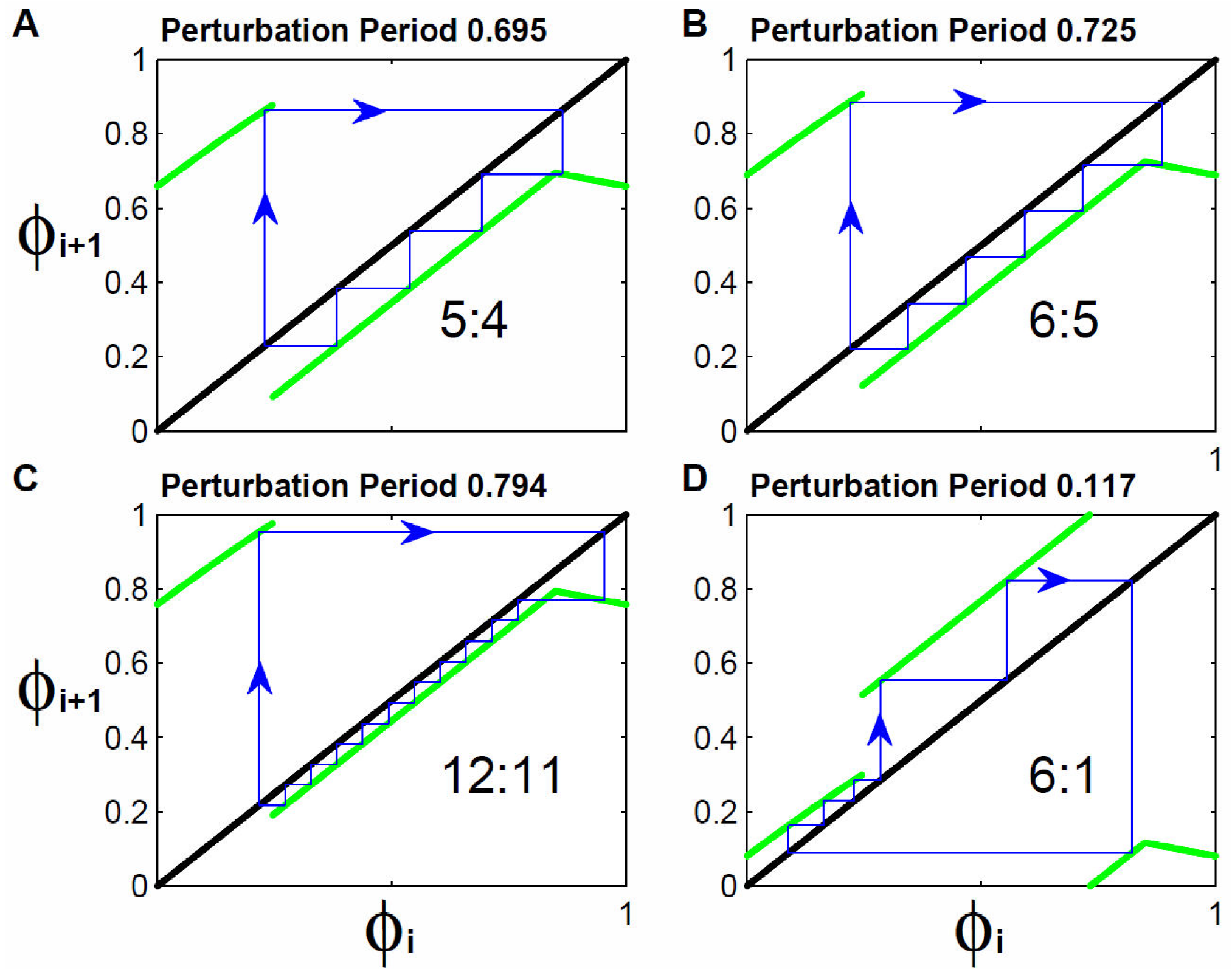
Figure 1. Experimental Device. The main element of the experimental device is a glass provided with a siphon inside it. The glass is fed with water at a constant rate of 5.27 mL/seconds, and as the water level increases the siphon is simultaneously filled. When the water reaches the maximum level of the siphon, the glass is rapidly emptied through it. This system is perturbed with water pulses two seconds long injected by means of a pump controlled by an Arduino board. The pulses can be either isolated or periodic. With label P1 the perturbation pump is indicated and with P2 the feeding one.
There is another tubing inside the container that corresponds to the perturbation hose; it is 9 mm in diameter and it is connected to a Comet Elegant submergible pump controlled by an Arduino board which is controlled by a PC. With this system, we apply water pulses whose volume can be adjusted by the voltage applied to the pump. Pulses can be isolated or periodically applied. Volume perturbations were given as fractions of the work volume, for example a perturbation of 0.1 corresponds to a volume of 46.9 mL.
Water level evolution was recorded by a Sony Digital video camera. To improve the resolution of the images, the water was stained with orange or blue dye. The video acquisition was done at 31 frames per second. Water levels were measured directly on the video recordings and also were analyzed with the free software ImageJ 1.48v by using the luminosity of the water mass, this measurement is proportional to the water height within the container.
2.2. Data Fitting and Simulations
The Tantalus device just described before was used to obtain the natural oscillation of the system. Ten oscillations were recorded to measure the water level evolution directly frame by frame. Data corresponding to three oscillations are shown in panel A of Fig. 2. We define the highest level of the water oscillations as the starting moment of the cycle, and name it marker event 6,7. By using the ImageJ program, we calculated the mean value for the period resulting 126.7 seconds with standard deviation of 1.24 seconds.
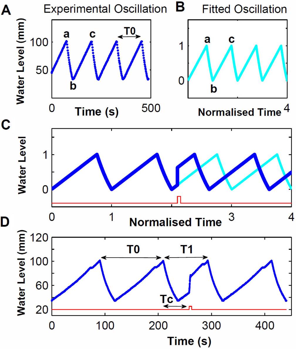
Figure 2. Natural and perturbed oscillations. Panel A. Display of an experimental oscillation. A measure was taken for every 30th of a second. It is considered a complete oscillation going through the points a, b and c. The natural period of the oscillation, T0, shown in this recording has a value of 126.3 seconds. Panel B. Graph of the adjustments to the normalized oscillation. The downward section was adjusted with a parabola, while the upward section with a straight line that reflects the constant rate at which the glass is filled. Panel C. Model of instantaneous perturbation when the water level is rising. The cyan trace shows what would have been the water level evolution if no perturbation was applied. The blue trace is the evolution of the water level resulting from the perturbation. The square pulse in red shows the moment in which the water was injected. It can be noticed that the effect of the perturbation is to reduce the time of the oscillation. According to the moment when the pulse is applied the oscillation can be lengthened, shortened or not present any effect. Panel D. Experimental recording of the effect of an isolated perturbation. T0 corresponds to the natural period of oscillation, T1 to the perturbed period of oscillation which in this case is smaller. Tc is the time elapsed between the “marker event” (corresponding to the beginning of the oscillation) and the water injection.
In order to fit a function to the water level evolution the experimental data were normalized dividing them by the natural oscillation period. Also the water level variations were normalized with respect to the maximal amplitude. The water discharge, indicated as “a-b” segment in panel A of Fig. 2 has a parabolic shape 20 whose mathematical relationship is given by:
Where N is water level, t is time; (t v , N v ) are the coordinates of the parabola vertex; 4p = 5.11, t v = 0.521 and N v = -0.39. The fitting function had a correlation R 2 = 0.996.
The fitting for the filling course of the Tantalus, “b-c” segment in panel A of Fig. 2 was done by means of the straight line:
Where m = 1.325 and b = -0.325. Panel B in Fig. 2 displays the normalized and fitted oscillations. The theoretical analysis reported in the following pages is based on these two data fittings. In panel C of Fig. 2 the fitting is used to represent the effect of a volume perturbation of 0.5 times the work volume (WV), and it is applied when the container is filling. The cyan trace corresponds to the unperturbed oscillation and, the blue trace that has been superposed corresponds to the perturbed oscillation. The thin red trace at the lower part indicates, with a square pulse, the moment of the perturbation. We are considering its effect as instantaneously moving upward the water level 0.5 WV. After this change the oscillator continues its evolution starting from the newly reached level. In this case the perturbation effect was to reduce the oscillation period. We will say that in this case the oscillator moved forward. Depending on the precise moment of the perturbation application, the oscillator advances or delays. Moreover there is even a moment with no effect.
To quantitatively measure the effect of isolated perturbations and to predict the periodical perturbations effect we calculated the PTC 6,7. The central idea for this calculation is that the perturbation instantaneously moves the oscillator from one moment in the natural oscillation to another one. The moment just before the perturbation occurs is called old phase
To predict the effect of periodical perturbations with a fixed period
Once we know the initial phase, iteration of this expression lets us know the system evolution after n perturbations. Also it lets us infer if there exist coupling rhythms between perturbations and the modified behavior of the oscillator.
2.3. Analytical Method to Find New Phases
To analytically find the dependence of the new phases in terms of old phases we have to consider that subject to perturbations the oscillator may exhibit three operation regions 1) from the beginning of the emptying to the beginning of the filling up. This corresponds to the “a-b” interval in panel A of Fig. 2, this set of phases will be called R_I; 2) from the beginning of filling up to the moment the perturbation initiates the emptying phase. This region will be called R_II; this region depends on the perturbation intensity; 3) from the end of the last described region up to the beginning of the spontaneously emptying, point “c” in panel A of Fig. 2, this set of phases will be called R_III. Given that to do the analytical calculations we only consider the times corresponding to one oscillation. We will take those times described by fittings (1) and (2) as phases.
As it was mentioned in previous section, we consider that both perturbations and its effect on the water level are instantaneous; in the same way the change from old phase to new ones occurs.
The water level N
o
, corresponding to the old phase
Where the specific form of N
o
function depends on the region that we are considering. The water level N
n
, corresponding to new phase
Where the specific form of N
n
function depends on the region that we are considering. If we add
We will use these expressions to get the relationship between the new phases and old phases. We have to remark that the functional relationship for N o and N n depends on the operation region we are considering. For R_I region the water level is decreasing before the perturbation, and after the perturbation it will continue decreasing. In these cases we will use (1). For R_II the water level will be increasing before the perturbation and will continue increasing after the perturbation. Here we will use (2). However, for R_III the water level will be going up before the perturbation, but after the perturbation it will start to going down. In this region we are going to use (1) and (2).
Rearranging the terms we have for each operation region:
2.4. Experimental Method to Find New Phases
There is a huge amount of publications indicating how to calculate new phases from experimental data 21. In panel D of Fig. 2 there is a scheme which has been obtained from an experimental recording to illustrate how new phases are calculated. The unperturbed period of oscillation is denoted byT0, the perturbed oscillation period is T1. The time interval between the marker event previous to the perturbation and the perturbation time itself is T c . The time interval between the perturbation time and the next marker event is called cophase. The old phase is T c /T0:
While new phase is cophase subtracted from T0 and normalized, resulting in
3. Results
3.1 Theoretical Phase Transition Curves (PTC)
PTC is the relation between old phases and new phases 6,7. Figure 3 displays a PTC obtained using the analytical expressions described above with varied intensity: 0.2 WV in panel A; 0.4 WV in panel C; 0.6 WV in panel E. Intensities are indicated in the right lower corner in each panel. In the first panel, R1, R2 and R3 indicate the three different branches in the map depending on the operation region. We can observe that branch R1 has a discontinuity which is induced by the module 1 operator; its position depends on the perturbation intensity. In fact, the discontinuity phase can be calculated, since corresponds to the moment when the descending water level returns to the maximal level. There is another discontinuity in this map, and it is present for all the Tantalus PTC.
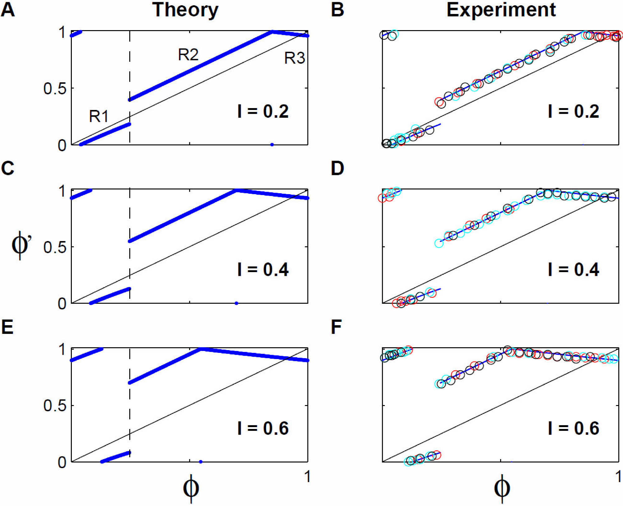
Figure 3. Experimental and Theoretical Phase Transition Curves. For all panels the horizontal axis indicates the old phase and the vertical axis the new phase. The panels on the left side correspond to the theoretical results and those on the right side to the experimental results. Each row corresponds to the same perturbation intensity, indicated on the lower right corner of each panel. The diagonal line is the graph of the identity function. In the theoretical panels the dotted line indicates the position of the map discontinuity which is insensitive to the perturbation intensity. Nevertheless, note that the magnitude of the discontinuity grows with the perturbation intensity. The maps are considered to be formed by three branches: R1, R2 and R3. In the experimental panels the different colors indicate experiments done on different days.
In the three left panels we have marked with a dotted thin line the moment when this discontinuity always occurs. In panel A the magnitude of this discontinuity is 0.22, up to two decimal ciphers; in panel C the magnitude is 0.42; and in panel E is 0.62. This means that the magnitude grows with perturbation intensity. This result can be analytically verified, obtaining the difference of new phase values, between the last point in branch R1 and the first of branch R2. This discontinuity, which we call “essential discontinuity”, occurs because before it perturbations delay the oscillator and, after it, perturbations advance the oscillator. This discontinuity will be the one inducing the BCB.
3.2. Experimental Phase Transition Curves
Following the procedure explained in Sec. 2.4 we did a set of experiments to measure the PTC for the same perturbation intensities as those theoretical results illustrated in Fig. 3A, C, E. Three runs were made on different days for each intensity. The perturbations were applied in five seconds intervals from the moment the container starts to fill and up to the moment it is empty, that is, during an entire cycle. Between consecutive perturbations two unperturbed oscillations were allowed. All this procedure was recorded by a digital camera, and to measure phases we took as a marker event the moment when the container starts emptying. Panels B, D and F in Fig. 3 show the corresponding results for 0.2, 0.4 and 0.6 WV intensities. Different colors represent different experiments done in different days. To facilitate comparison theoretical PTC are superposed. The coincidence between them is remarkable.
3.3. Periodical Rhythms: Theoretical prediction
To explore the dynamical evolution of the system we can choose any intensity, initial condition and a perturbation period using the function (8). In most of the cases we found that orbits converge to in fixed points or periodic orbits, that is, after certain number of perturbations the phases where the system moves around are the same. This repeated phases can be reached in one or several oscillations. The combination of the number of perturbations with the number of oscillations will be called coupling rhythm, and will be identified with N : M notation; where N = number of perturbations and M = number of oscillations. When two rhythms have the same N, we would say that they have the same periodicity.
Figure 4 shows some orbits obtained with 0.5 WV perturbation intensity. Panel A displays the orbit the system follows when 0.7T0 perturbation period and an initial condition of 0.32T0 were used. It can be seen that after a transient course of five iterations, the orbit converges to a point where the identity line intersects the map. Staying in this point means that before each perturbation the system is always at the same phase. This is a rhythm with 1-periodicity. This type of evolution occurs because the intersection of identity line with the map has an absolute value slope lower than one, in consequence, all orbits passing around that vicinity are attracted. This fact allows us to analytically calculate those 1-periodicity cases.
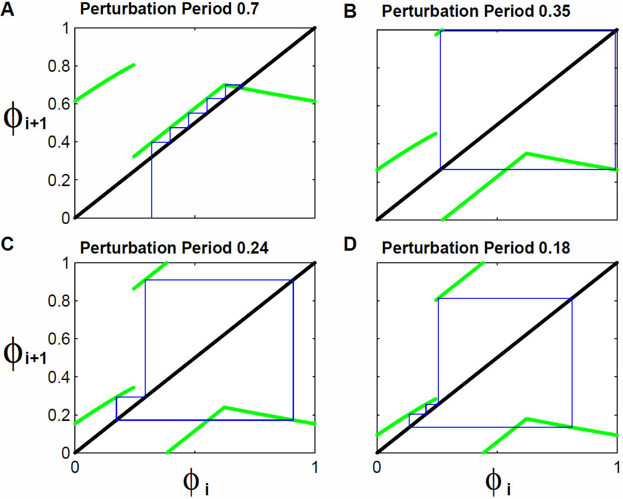
Figure 4. Resulting orbits from iterating the Phase Transition Curve for perturbation intensity of 0.5 WV. Panel A. Resulting orbit from iterating with a perturbation period of 0.7T0 and initial condition 0.32T0. After some iterations the orbit move to the crossing of the map and the identity function. A rhythm with 1-periodicity results given that each iteration falls in the same phase. Panel B. Orbit with 2-periodicity, resulting from iterating with perturbation period of 0.35T0, the orbits visit two phases of the map. In this panel, as in the following ones, the initial condition is omitted and only the asymptotic part of the orbit is illustrated. Panels C and D. Orbits with 3-periodicity and 4-periodicity resulting from iterating with perturbation periods of 0.24T0 and 0.18T0.
Panels B, C and D illustrate rhythms with higher periodicity, though transitory paths have not been represented, only the final orbits. Panel B presents a 2-periodicity rhythm obtained when perturbation period is 0.35TO. Panel C shows a 3-periodicity orbit occurring for perturbations applied 0.24T0 and, D a 4-periodicity orbit obtained for 0.18T0. It can be observed that between identity line and RI branch in the map there is a channel, and by adequately choosing the perturbation period it can be made as thin as desired. Reduction in the width of this channel will induce very long orbits.
3.4 Periodical Rhythms. Experimental results
To corroborate the theoretical predictions established in the last section, we perturbed the Tantalus oscillator with an intensity equal to 0.5 WV, which matches the case shown in Fig. 4. This means that volume pulses of 234.5 mL are injected in 2 seconds. In all the experiments the initial condition or first perturbation pulse phase was selected among the several points in the studied orbits. Then for perturbation period 0.7TO the first pulse was applied in phase 0.68T0. Panel A of Fig. 5 shows that the result in this case is a coupling with 1:1 rhythm. Panel B in the same figure shows the result for 0.33T0 perturbation period and an initial condition of 0.27T0, the obtained rhythm is 2:1. In panel C the coupling rhythm is 3:1, a result from perturbing with a 0.24T0 period and an initial condition of 0.17T0. Finally, in panel D a coupling rhythm 4:1 produced by perturbation pulses with 0.17T0 period and initial condition 0.81T0 is shown. Once again the coincidence between theory and experiments is remarkable. Not only are the predicted rhythms obtained; but they can also be reached by starting the perturbation protocol in the predicted phases. It has to be noted that each experiment was repeated at least three times.
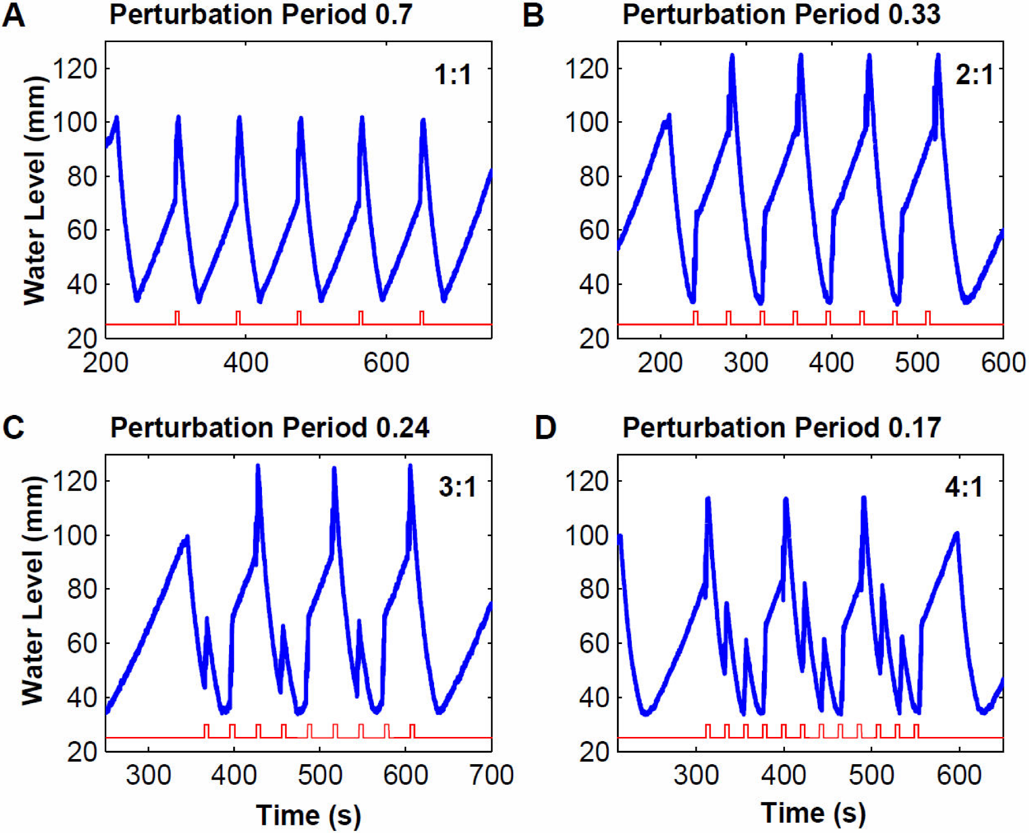
Figure 5. Resulting couplings from applying periodic perturbations with intensity 0.5 Experimental recordings resulting from applying periodic perturbations with periods and intensities as in Fig. 4. Points of the theoretically calculated orbits were taken as initial conditions for each experiment. In each panel the horizontal axis indicates time in seconds. In the vertical axis indicates the water height in millimeters. In the upper part of each panel the perturbation period and resulting rhythm is indicated, where the first digit indicates the number of perturbations and the second one the number of oscillations in which the patterns is repeated.
3.5. Bifurcation Diagrams for the Perturbation Period
By repeating the exercise that we have described in Sec. 3.3, but now for intensities going from 0.1 to 1.05 in 0.01 step size; for 1000 periods between 0 and 1 with 0.001 steps size and for 10 initial conditions between 0 and 1 with 0.1 steps size, we completed 950 000 studied cases. We looked for periodicities between 1 and 16 making 2560 iterations in each case. Most of the cases: 871 211 had periodicity between 1 and 16. The remaining cases could have longer periodicities. In Fig. 6, panels A and B, we show the periodicities pattern obtained for perturbation intensities 0.2 WV and 0.4 WV. It can be seen that the periodicity patterns have a general horseshoe shape, built by rungs that constitutes a staircase. At the right and left ends, outside the horseshoe, there are 1-rhythm regions; these rhythms are consequence of the intersection between the identity line and the mapping, as has been described in Sec. 3.3. As perturbation intensity grows these regions grow, which reflects that R3 grows with the perturbation intensity, as can be seen in the left panels of Fig. 3.
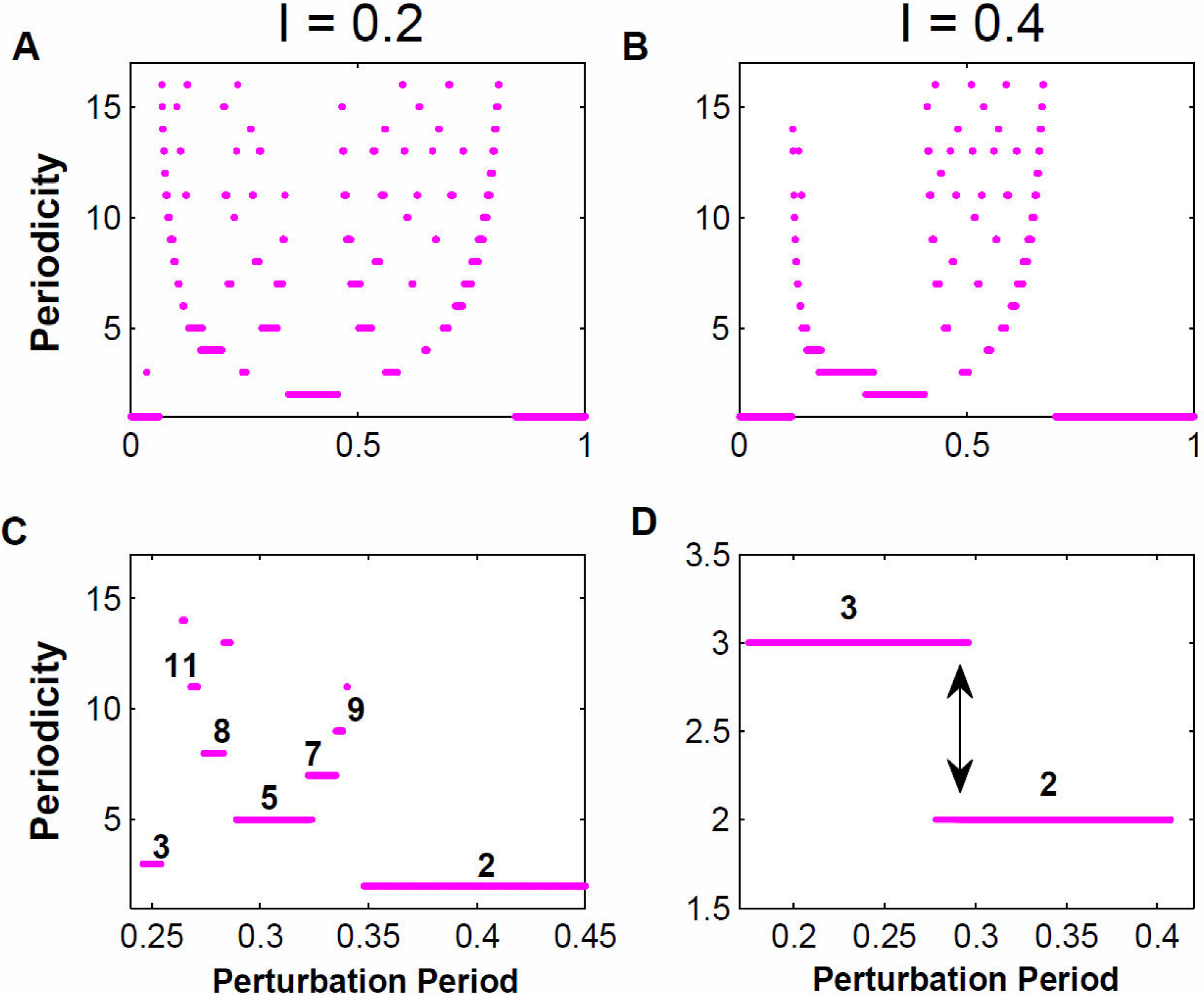
Figure 6. One-parametric Bifurcation Diagrams: increasing, additive and with bistabilities zones. In panels A and B are shown the bifurcation diagrams obtained when perturbing with periods between 0 and 1, in steps of 0.0001. In the first panel the perturbations are done with an intensity of 0.2 WV and in the second one of 0.4 WV. Panel C. Detail of panel A, for periods between 0.25T0 and 0.45T0. It can be noted that between the regions with 2-periodicity and 3-periodicity there exists a gap filled with periodicities that sum the periodicities of the edges, this way we have a region with periodicity 3+2=5, another one with 3+5=8, etc. Panel D. Detail of panel B, for periods between 0.17T0 and 0.42T0. It can be noticed that region of 2-periodicity and the one of 3-periodicity overlap, which predicts the existence of bistabilities.
In general, we have “additive periodicities”, that is, consecutive periodicities do not have contiguous domains of rhythms 22. This characteristic is illustrated in panel C of Fig. 5. Here we show that between 2-periodicity and 3-periodicity there is a gap. This gap is partially occupied by a 2 + 3 = 5-periodicity region. Between 2-periodicity and 5-periodicity zones there is a 2 +5 = 7-periodicity zone; and so on and so forth. Panel D in the same figure shows another type of phenomena commonly found in Periodicity Diagrams or One-parametric Bifurcation Diagrams. In the region between perturbation periods 0.2T0 and 0.4T0 and perturbations intensity 0.4 WV, there is a region in which when changing the initial condition, we get different coupling rhythms, that is, there is bistability and this property is very common in the Tantalus Oscillator diagrams.
3.6 Experimental verification of Bistability and Additive Rhythms
In panel A of Fig. 7 we show a 2-rhythm coupling obtained by using a perturbation period of 0.4T0, we have two perturbations for each Tantalus oscillation. Repeating the procedure for perturbation period 0.25T0 we get a 3-rhythm coupling, three perturbations for one Tantalus oscillation, this is shown in panel B in the same figure. Finally, when we chose an intermediate perturbation period, 0.3T0, which according to the results displayed in panel C of Fig. 6 should correspond to a 5-periodicity pattern, we see that the experimental result is five perturbations coupled to two Tantalus oscillations.
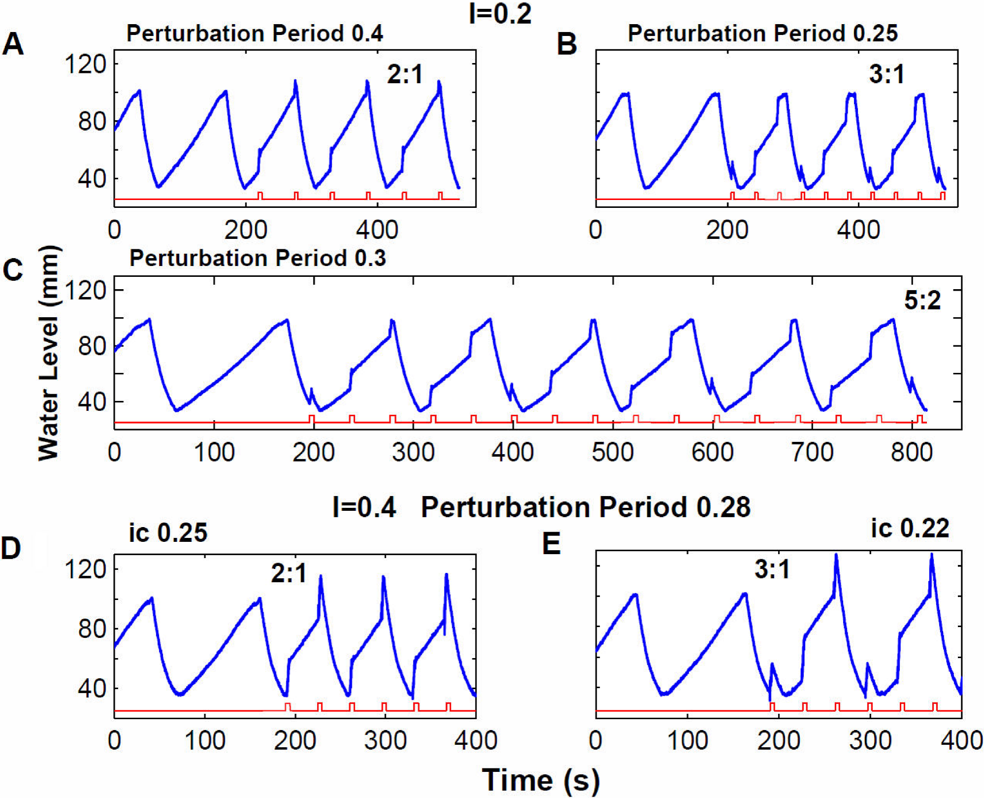
Figure 7. Experimental recordings: additive and bistable rhythms. In the first three panels the addition phenomenon is illustrated, obtained with a perturbation intensity of 0.2 WV. In the last two panels the bistability phenomenon is illustrated, obtained with a perturbation intensity of 0.4 WV. In all the panels the blue trace shows the evolution of the water level, the red trace indicates the perturbation moments. Panel A. Rhythm 2:1 obtained with a perturbation period of 0.4T0; we have two perturbations per oscillation. Panel B. Rhythm 3:1 obtained with a perturbation period of 0.25T0; we have three perturbations per oscillation. Panel C. Applying perturbations with period in between the previous ones: 0.3, a rhythm 5:2 is obtained, which is the combination of the elemental blocks for 2:1 and 3:1. We have 5 perturbations in two oscillations. In panels D and E perturbations with the same intensity and period were applied: 0.4WV and 0.28T0. In panel D the initial condition was 0.25T0 and the resulting rhythm was 2:1. In panel E the initial condition was 0.22T0 and the obtained rhythm 3:1.
In relation to the experimental verification for the existence of predicted bistabilities (panel D of Fig. 6), we have explored for perturbation intensity 0.4 WV and different perturbation periods overlapping their respective regions. In panels D and E of Fig. 7 we show the results obtained after applying repetitive pulses with a perturbation period of 0.28T0 and initial condition of 0.25T0 (panel D) and the same parameters values but with initial condition 0.22T0 (panel E). It can be observed that we get two different couplings: 2:1 and 3:1.
3.7. Border Collision Bifurcations
Bifurcation Diagrams described in the previous paragraph in which the system “jumps” from one periodicity to another pose the question: what kind of bifurcations occur between one periodicity and the other? In most cases we are studying the bifurcations type is Border Collision and it happens because the orbits collide with the essential discontinuity described at the beginning of this results section. In Fig. 8 we illustrate how this kind of bifurcation occurs when the perturbation intensity is 0.2 WV, perturbation period goes from 0.182T0 to 0.154T0 and the initial condition is 0.1. In panel A the 4-period orbit when perturbation period is 0.182T0 is shown.
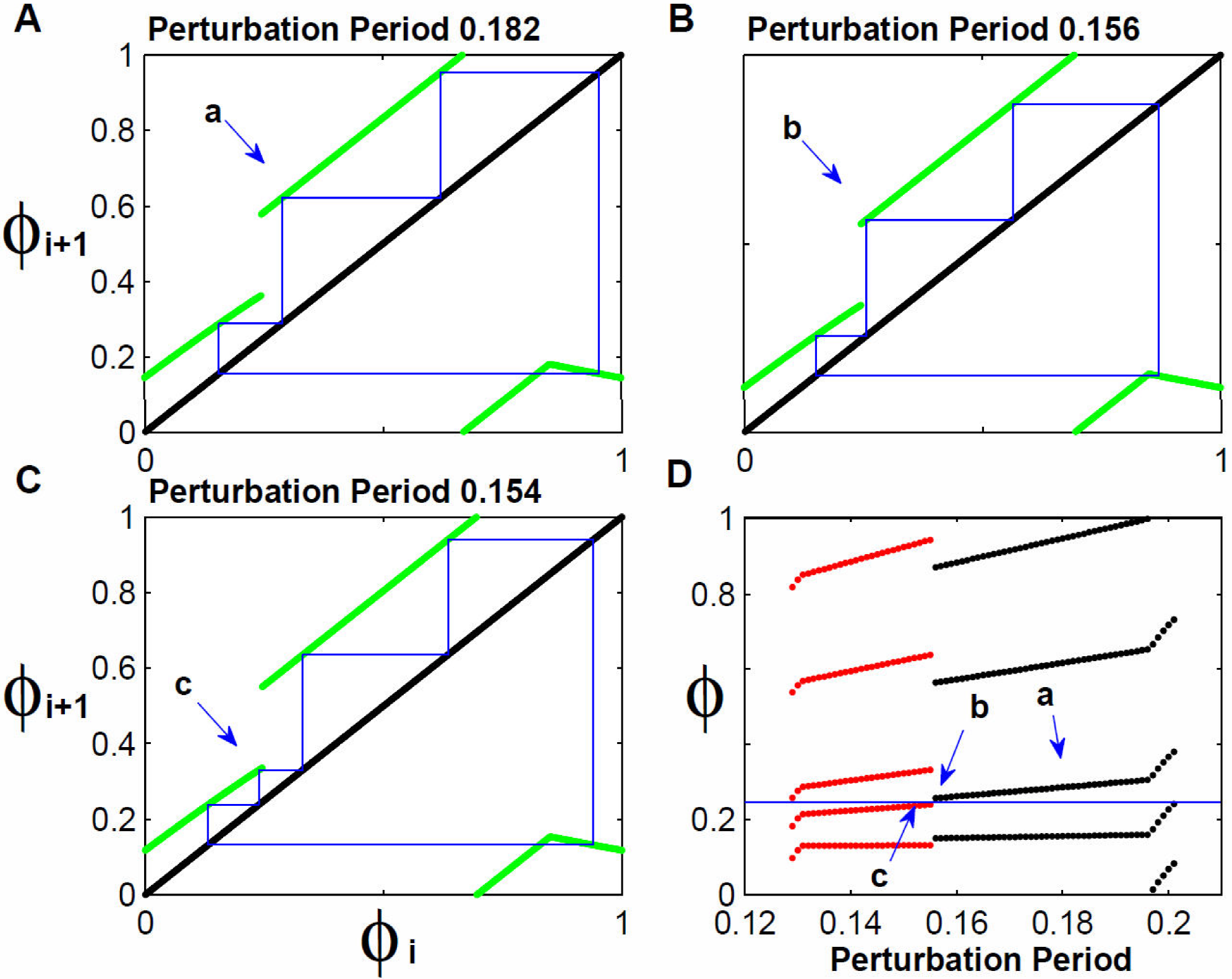
Figure 8. Border Collision Bifurcations. Transition between 4-periodicity and 5-periodicity during the period reduction. In Panel A the obtained orbit for a perturbation period of 0.182T0 is shown; it has 4-periodicity. The third element of the orbit is identified with a blue arrow and the letter “a”. Panel B. The reduction the perturbation period to 0.156T0 approaches this third element to the map discontinuity, now marked labeled with letter “b”. Panel C. A very small reduction makes the third element of the map collide with the map discontinuity and reorganizes the orbit with now five elements. Panel D. In the horizontal axis the perturbation period is indicated, in the vertical axis the phases the iteration visits are indicated. Phases with 4-periodicity are in black and those of 5-periodicity in red. The horizontal blue line indicates the discontinuity position. Observing the graph from right to left it can be seen that the 4 periodicity starts in the fourth phase and ends in the third one. At that moment the 5 periodicity starts in its fourth phase to end in its third one. We are counting the phases from top to bottom.
The arrow and “a” letter are indicating one of the four elements in the orbit. As the perturbation periodicity is decreasing, this element is approaching the discontinuity. In panel B we see its new position indicated with an arrow and “b” letter, when the perturbation period is 0.156T0. At that moment it is almost touching the discontinuity. Another small reduction in the perturbation period causes the orbit to touch the discontinuity and moves from branch R2 to branch R1, reorganizing the orbit path that now has 5-periodicity. In panel D of the same figure, we show in a general fashion these bifurcations. We plot the phase values for each orbit element for perturbation periods from 0.12 to 0.2. In red we show phase values corresponding to 5-rhythm, in black the phase values corresponding to 4-rhythm. A thin horizontal blue line marks the essential discontinuity position; arrows indicate the position of a, b and c points marked in panels A, B and C. If we analyze the pattern of moving phases going from right to left along the blue line, we can see that 4-rhythm begins at the discontinuity point for the fourth phase (if considered from top to bottom), and it finishes to the end of third phase in the same discontinuity line. For the fourth phase, the 5-periodicity rhythm emerges which ends in the same discontinuity for the third phase.
A detailed inspection of the phase diagrams for each studied perturbation intensity and for each initial condition shows all bifurcations occur in this way when we plot the phases between 0 and 1. Then we can say that most of the bifurcations occurring in this system are BCB, without discarding that there may be some other bifurcation types.
3.8 Two-parametric Bifurcation Diagram
We can group the One-parametric Bifurcations Diagrams as those shown in panels A and B of Fig. 6, to build a TBD. In panel A of Fig. 9 this construction is shown. The horizontal axis indicates perturbation periods from 0 to 1 in step size of 0.001; in the vertical axis we represent the perturbation intensity between 0.1 and 1.05 WV in step size of 0.001; in total we have 950 000 points. Periodicities up to fourteen are represented giving the same color to these rhythms with the same periodicity. It can be seen that in general, the diagram has the same appearance as those obtained by Chialvo 18 and Santillán 19. There are large zones with 1:0 and 1:1 rhythm at both sides. The region with higher rhythm has a triangular shape with its vertex pointing towards higher intensities. The border zone with 1:0 rhythms is barely curved, while the border with the 1:1 region is a straight-line.
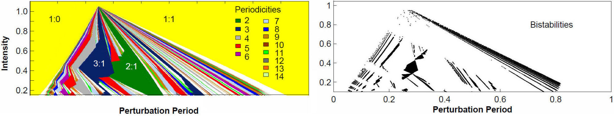
Figure 9. Two-parametric Bifurcation Diagram and Bistabilities Diagram. In both panels the horizontal axis indicates the periodicity and the vertical axis the perturbation intensity. Panel A. Regions with similar periodicity are indicated with the same color. Yellow for periodicity 1. White regions have periodicity greater than 14. Panel B. Regions with different periodicities overlap, this indicates that there are many bistability regions. These regions are indicated in black.
The pattern inside the triangle is formed by bands, that is, sets of points with the same rhythm. As some of the rhythms share the same periodicity, we assigned all of them the same color. For example, looking at the diagram from left to right we see 5:1, 5:2, 5:3 and 5:4 rhythm bands. To all of them we assigned the red color. At the right side of the figure it appears the color code for periodicities, reported up to 14. Yellow color corresponds to 1-periodicity. On the left side of the figure is the 1:0 coupling, meaning that the system receives periodic perturbation in the same phase but never completes an oscillation. On the right side the coupling is 1:1, implying an oscillation is produced for each volume perturbation applied in the same T0 phase.
Although the diagram changes as the intensity perturbation grows, there are some general characteristics. A notable one is that periodicities accumulate to the left and right of the diagram boundaries. In both cases, as we approach to the borders, longer periodicities are observed, but each time in narrower zones. This property could be observed in the One-parametric Bifurcation Diagrams of panels A and B of Fig. 6. Another general characteristic is that a band rhythms goes to the vertex of the triangle becoming thinner but preserving their ordering. Zooming the visualization of the diagram at different heights, the same band ordering is observed. A novel result respect to Chialvo and Santillán 18,19 papers, is the existence of bistabilities in our system. In panel B of Fig. 9 they are shown. We can see that besides a wide zone between 2:1 and 3:1 rhythm; in the middle of the diagram there are bistabilities too. They accumulate towards the boundaries. White zones in the diagram are partially ought to bistabilities of very high order not detected in our simulations.
4. Discussion
There is a large number of oscillators that can be typified as oscillators with a stable limit cycle. Among those, some of them can be modelled by discontinuous PTC’s under brief perturbations, the Tantalus oscillator being one of these. This oscillator had already been studied from the nonlinear dynamics perspective by Chialvo, et al. 18 these authors showed that by changing the perturbation period it can be found that the Periodicity Diagram has a Devil’s Staircase shape.
Besides considering the perturbation period as a bifurcation parameter, its intensity is also considered, then triangular coupling regions can be found for periodicities greater than 1, though for big perturbation intensities rhythms 1:0, 2:1 and 1:1 still remain, this being due to the model characteristic that does not allow the water level to go over the maximal threshold regardless the moment when the perturbation takes place.
In 2016 a paper was published 19 dealing with a system analogous to the Tantalus Oscillator in which results similar to those in Chialvo, et al. are obtained. In that case it is a capacitor being charged until it reaches its threshold voltage and when it does so, it discharges rapidly 19. The voltage oscillation has a shape very close to the water level in the Tantalus Oscillator. The charge and discharge process can be affected by a circuitry which allows introducing constant period voltage pulses. Even though with that systems it is not possible to evaluate the effect of isolated perturbations, the author manages to extract a PTC by means of studying the effect of individual pulses from the train of stimuli.
Among the presented results it can be highlighted a TBD. This diagram displays periodicities according to perturbation period and intensity; and its shape is very close to that obtained by Chialvo, et al. Nevertheless, it is shown by the author as well; that in the studied case, all rhythms with periodicity greater than one converge to one point. It also happens that, since the origin of all oscillations (and the marking event to calculate the PTC’s) is defined as the moment when the capacitor is starting the charging process, the discontinuity characteristic is less noticeable.
In our case we have taken the beginning of the emptying process of the Tantalus Oscillator as the origin of all oscillations, and also as marking event. This highlights the phase where the isolated perturbation PTC’s obtained have their discontinuity. This discontinuity is precisely where the orbits collide when the perturbation period is changed and produces a BCB. These bifurcations are the dominant ones in the bifurcation diagram. Besides, a variety of phenomena occur as the perturbation period and/or intensity are modified. These phenomena have been shown and discussed in several theoretical papers regarding discontinuous maps. One of the research groups that has more contributed in the study of these phenomena is the group leading by Avrutin 16,17,22,23,25. We will discuss the trajectory reinjection mechanism happening in the Tantalus map. This mechanism was addressed, in general, in a paper of the mentioned research group in the year 2000 23. Supported on that work we propose that the peak of the rhythms with periodicity greater than one in the two-parametric diagram is a point where a BBB takes place.
The reinjection mechanism was suggested by Pérez in 1985 24 and developed by Avrutin in 2000 23. For this aim the following map was used:
The dynamic associated with this discontinuous map includes countless periodic orbits. It consists of a line parallel to the identity function separated a distance “a” from it, and of a small horizontal segment on the abscissa axis. The domain section where the first segment of the map is valid is [0,1) and the second part applies for the values greater than or equal to one. The orbits this map induces, consist on a series of steps formed in between the identity function and the diagonal section of the map, see Fig. 2 Ref. 23. When the orbit attains a value in the interval [1-a,1) the value for the next iteration is zero and the orbit repeats itself. This is the mechanism known as reinjection. The number of steps depends on the value “a”, the lower it is the larger the number of steps and the greater the periodicity of the orbit. As it can be seen with this map, a countless number of periodic orbits can be generated.
A similar mechanism exists with the map obtained for the Tantalus oscillator. In Fig. 3 it can be seen that any perturbation intensity studied forms a channel between the PTC and the identity function. In Fig. 4 it can be seen that the magnitude of the perturbation period modifies the width of the channel and the size and organization of the orbits. For instance, for perturbation periods close to zero or one there exists an intersection between the identity function and the branch R3 of the map, therefore there are no channels formed. Nevertheless, when the period moves the map upwards or downwards, the previously mentioned crossing is eliminated and therefore stepped orbits can be found for which the reinjection mechanism occurs. This is shown in Fig. 10. In panel A we show the orbit occurring for a perturbation period of 0.695T0. In this case branches R2 and R3 form a channel with the identity function in which the orbit will move. The value of the perturbation period is such that it allows the formation of four steps before the orbit leaves through the lower side of the channel and travels to the branch R1 where it reinjects to traverse once again the channel. If a simulation of the water level is done for this case, a pattern is found to be repeated four times for every five applied perturbations, this being a rhythm 5:4. If the perturbation period is slightly increased the width of the channel is reduced. In panel B we show that for Tp = 0.725T0 the new channel width compels to traverse it in five steps. The organization of the orbit is exactly the same as discussed above but with an additional step, therefore the rhythm obtained is 6:5, that is, five oscillations where six perturbations fall. The range of this procedure seems to be limitless regarding the number of steps that can be fitted. In panel C we increase the perturbation period to 0.794T0, the channel width is once again reduced and to traverse it eleven steps are needed, this way we get a periodicity rhythm of twelve. It must be mentioned that we have illustrated the type of channel formed for perturbation periods greater than 0.5 WV, but we shall mention that for periods lower than 0.5 WV a similar channel is formed but it does in between the branch R1 and part of the branch R2, as shown in the orbit with periodicity 6 occurring for Tp = 0.117T0.
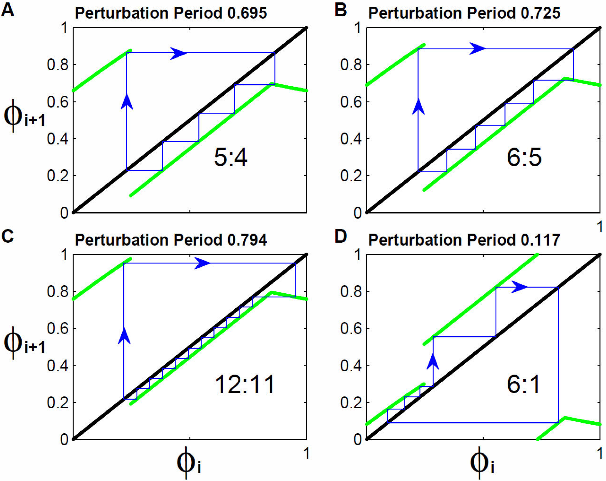
Figure 10. Reinjection mechanism for the Tantalus map. For low or high periodicities, the map forms a channel with the identity function through which the orbit flows. In the case of high periodicities, the channel is formed by branch R2 and the orbit is reflected in branch R1 to be reinjected in the channel. In panels A, B and C it is shown that as the perturbation period increases, the channel is narrower, the orbits have more steps and the periodicity is higher. This mechanism works for any length of branch R2, that is for any perturbation lower than 1. In panel D it is shown that the same mechanism also works for brief perturbation periods.
Relying on the reinjection mechanism we infer that the peak of the TBD, in its periodicities greater than one, is a BBB. Recalling that a BBB is a point in which an infinite number of bifurcation lines converge. In this case, the bifurcation lines would be of border collision. This lines would be induced by the reinjection mechanism occurring basically in a channel formed between the identity function and the map. The orbit traverses this channel through a given number of steps and then leaves it to be reflected somewhere else in the map where it only suffers from one iteration. In the case of high periodicities, as shown in panels A, B, and C of Fig. 10 the number of steps gone through depends on two factors: the existing distance between branch R2 of the map and the identity function (distance determined by the perturbation period) and the length of the branch R2 of the map (determined by the perturbation intensity). Therefore, as long as the perturbation intensity is less than one the branch R2 of the map it will have a length different from zero which will allow the generation of orbits with periodicities as lengthy as wanted, for which it would only be required to approach the map and the identity function as much as needed.
As we have shown through the results, the regions of differentiated periodicities are separated by BCB. When the perturbation intensity becomes 1, the branch R2 of the map, as well as the essential discontinuity and all the rhythms with periodicity greater than 1 disappear simultaneously. We infer that at that moment a BBB takes place. A similar result for other maps has been discussed in Ref. 25.
5. Conclusions
The Tantalus oscillator is a nonlinear oscillator with stable limit cycle. It is of hydraulic nature and its oscillation period depends on the filling and emptying rates as well as on the container’s volume with which it is constructed. When this system suffers brief perturbations it returns to its original oscillation after a short transient. In this research we apply monophasic perturbations to a Tantalus oscillator, those perturbations being injections of a given volume of water. The injected volumes are smaller than the volume of the container and their duration is shorter than 2% of the normal oscillatory period.
We have done the analytical calculation of the PTC’s linked to these perturbations. We found that this curve has a discontinuity, which we have named essential, which exists for all the perturbation intensities smaller than the actual volume of the container. The size of the discontinuity increases with the perturbation magnitude. We experimentally measured the PTC’s and found an extraordinary consistency with the curves analytically predicted.
We iterate the PTC’s to predict the effect of periodic perturbations, varying the period for fixed given volumes of perturbation. We find bifurcation diagrams with the shape predicted by Avrutin, et al. for discontinuous maps, those authors named these diagrams Periodicity Diagrams. In our case these are increasing, additive and with bistabilities 22. We experimentally show some of the rhythms illustrated in the research, Figs. 5 and 7. We show experimental occurrence of bistabilities and the oscillation patterns matching the addition of periodicities.
We study the type of occurring bifurcation between both periodicities and find they are BCB. The same behavior changes take place when some of the elements of the orbit “collide” with the discontinuity in the PTC’s. We construct the TBD finding it has the general form as the one found in Chialvo, et al. for the Tantalus oscillator 18 and by Santillán for an analogous system 19. Nevertheless, in our case it is possible to notice a large number of bistabilities. It is also observed that towards the frontiers of the rhythms 1:0 and 1:1 the periodicity of the rhythms increases, leaving the regions of different rhythms split by BCB. This is due to the reinjection mechanism discussed by the Avrutin research group for discontinuous maps 23. Based on this mechanism, we infer that the number this BCB lines are infinite. Given that they converge in only one point of the TBD, and they do so in a point where the map loses its discontinuity, we infer that this point is a BBB, since it has been shown that for a similar system, whenever the map ceases to be discontinuous a BBB takes place 25.

