1. Introduction

Fractional quantum mechanics has been of great interest by many researchers recently. Laskin¹ has developed fractional generalization of the Schrödinger equation, Dong and Xu² used a new equation to study time evolution of the space-time fractional quantum system in the time-independent potential fields. Dong³ solved Schrödinger equation with infinite potential well using Levy path integral approach, where he obtained among other things the even and odd parity wave functions. Narahari et al⁴ presented a survey of several approaches that have been proposed to solve the fractional simple harmonic oscillator. He discussed the advantages and disadvantages and proposed a generalization of the integral equation of the simple harmonic oscillator that involves physically meaningful initial conditions. Rozmej and Bandrowski⁵ and Mahata⁶ discussed some applications of a fractional approach to the Schrödinger equation. Herrmann⁷ investigated fractional derivative in Schrödinger equation with an infinite potential well. Ibrahim and Jalab⁸ introduced analytical and numerical solutions for systems of fractional Schrödinger equation using Riemann-Liouville differential operator. Laskin^9,10 applied fractional calculus to quantum mechanics. He studied the properties of fractional differential equation and applied it to a Hydrogen-like atom. Guo and Xu¹¹ solved the fractional Schrödinger equation for a free particle and for an infinite square potential well and obtained the energy levels and the normalized wave functions. Many applications of fractional quantum mechanics can be obtained in Herrmann¹², Kilbas et al¹³ and fractional differential equation can be found in Podlubny¹⁴.

In all the aforementioned works the authors dealt with the second derivative concerning the kinetic energy. They converted the second derivative to a fractional derivative and showed its effect on the wave function and eigenvalues of the energy. In this work we will demonstrate the effect of an evolved electric potential on a charged particle placed in a harmonic oscillator; the potential is developing instead of growing. The derivative in this work is kept unchanged. The idea of evolution of some physical phenomena has been studied using fractional calculus to give deeper understanding of physical phenomena. It was possible to do so through varying the order of fractional differentiation from zero to one and observing the change in the phenomenon under consideration, and observe how it develops from one state to the other through the fractional operation. Engheta^15,16,17 applied the idea to the electromagnetic multipole showing the evolution of multipole from a certain order to the higher one. Rousan et al¹⁸ have studied such evolution in gravity and showed the evolution of a semi-infinite linear mass from a point mass. Rousan et al¹⁹ showed how the oscillatory behavior (LC circuit) goes over a decay behavior (RC circuit) as the order of fractional differentiation goes from zero to one, and vice versa. Also Rousan et al²⁰ studied fractional harmonic oscillator and suggested that the system goes through an evolution process as the fractional order goes from zero (free) to one (damped), letting it pass through intermediate stages where the system can have a damping character and the material can be thought as a pseudo-damping material. Gómez-Aguilar and co-workers contributed intensively to the field of fractional calculus. They studied fractional electrical circuits. They introduced an analytical solution to LC, RC, RL and RLC circuits in terms of the Mittag-Leffler function depending on the order of the fractional differential equation^21,22. Also they studied the transitory response and analyzed time and frequency domain of RC circuit applying Caputo fractional derivative^23,24. Moreover they described the dynamics of charged particles in electric fields employing Laplace transform of Caputo derivative²⁵. They also used Fourier method to find the full analytical solution of electromagnetic wave in conducting media considering Dirichlet conditions²⁶. Fractional electrical circuits were studied and analyzed from all aspects by Kaczorek and Rogowski ^27,28. Obeidat et al²⁹ studied the evolution of a current in a wire and estimated the time required for the current to reach its maximum value. A full review of the scope of applications of fractional calculus in physics and its applications on evolution process is found in¹⁸.

2. Method

The one dimensional time independent Schrödinger equation is given by:

Where m is the mass of the particle influenced by the potential V(x), ℏ is the normalized Plank’s constant, E is the energy of the system and ψ is the wave function. For harmonic oscillator, the restoring force on the mass is F=-kx, where k is the restoring force constant. The above equation (Eq. 1) reduces to

This equation has a well-known solution given in many quantum mechanics text books as ³⁰

Where ξ=(mω/ℏ)2x, and ω=k/m is the frequency of the oscillator, and Hn(ξ) is the Hermite polynomials of degree n. The quantized energy of the oscillator is given by:

If we assume the particle has a charge q and the above oscillator is placed in an electric field of strength ε, then the modified Schrödinger equation becomes

Complete the squares, the above equation reduces to

With

And

So, the solution again is the same as the normal harmonic oscillator but with a shift in the displacement and with modified quantized energy.

In this work, we suggest a potential of the form

Where α takes the values from 0 to 1 to be introduced to the oscillator, Schrödinger equation will be then written in the form:

The factor x01-α is introduced here for dimensionality.

There exist exact solutions for the limiting values of α namely zero and one, while for the intermediate values of α a numerical solution utilizing Numerov Algorithm will be used. Even though, the Runge-Kutta (RK4) method is a very powerful technique to solve ordinary or system of ordinary differential equations numerically, the Numerov Algorithm still is the simplest and most powerful accurate algorithm in solving such kind of problems even for central potentials. Numerov algorithm was proven to be faster and more stable^31,32. The error using Numerov algorithm on each step, h, is of order O(h ⁵ ), while the error using the Runga-Kutta (RK4) method is of order O(h ⁴ ), i.e., one order of magnitude better. Due to problems of round off error in Eq. (13), double precession arithmetic is used. Applying Numerov method to the general form of the second order differential equation of the form

Where (g)x and s(x) are known functions, with initial conditions given by y(x0)=y0 and y'(x0)=y0', in our case

and s(x)=0, the final form of Numerov´s formula is

With

Δx is the step. Complete derivation for Numerov Algorithm and final formula can be found somewhere else³³.

The values of constants throughout this work will be considered as:

3. Results and Discussion

The idea of this work is to demonstrate the effect of an evolved electric potential on the charged particle placed in a harmonic oscillator; the potential is developing instead of growing.

We first consider the wave function. As for the case of no electric field, which means that the value of α in Eq. (10) is zero which represents Eq. (2), and the case when there is an electric field (well developed) which means that the value of α in Eq. (10) is one which represents Eq. (5). It is expected now that as the value of α increases from zero to one the wave function shifts to the right. The way that the evolved potential affects the wave function is demonstrated in Fig. 1 where the wave function is displaced to the right towards a fully developed potential (α=1) as expected.

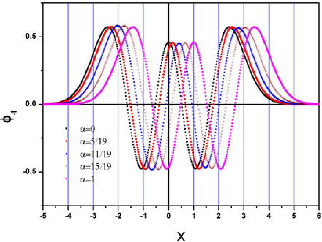
Figure 1. The figure shows the wave function (n = 4) for different values of α. The wave function shifts to the right as α increases. 

Taking the range of x from -5 to +5, the wave function for the case of n=4 for different values of α, Fig. 1 shows, beside the shift to the right the amplitudes seam to change slightly without indicating a specific trend which we believe due to normalization. Since the values of x ranging from a negative value to a positive value, care must be taken in choosing the values of α. In our case, we limited the values to be of power an odd number divided by an odd number.

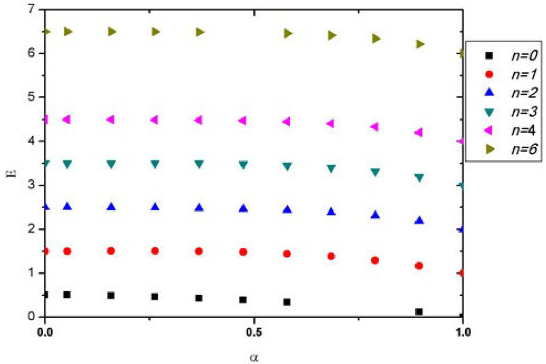
The values of energy are plotted versus α for different values of n in Fig. 2, where the values of energy decrease smoothly from that belong to the simple harmonic case (α=0) to that of applying the “full” potential (α=1), which is expected.

Figure 2. The energy of the system as a function of α for different values of the quantum number n. 

It might be useful to show how the potential itself is being developed as α increases from zero to one. We first show the potential for α=0 in Fig. 3 and that for α=1 in Fig. 4. The evolution then will be between those two limiting cases. Figure 5 shows the potential for selected values of α where a discontinuity appears in its derivative at x = 0, indicating the evolution process which affects the wave function. This discontinuity vanishes as α approaches unity as expected. In this process the potential shifts the minimum along the x-axis where the potential in this case is the total potential combining the harmonic oscillator and the electric potential. It is clear that the potential reshapes itself gradually between the two limits of α.

Figure 3. The potential for α=0. It represents the harmonic oscillator potential with no field. 

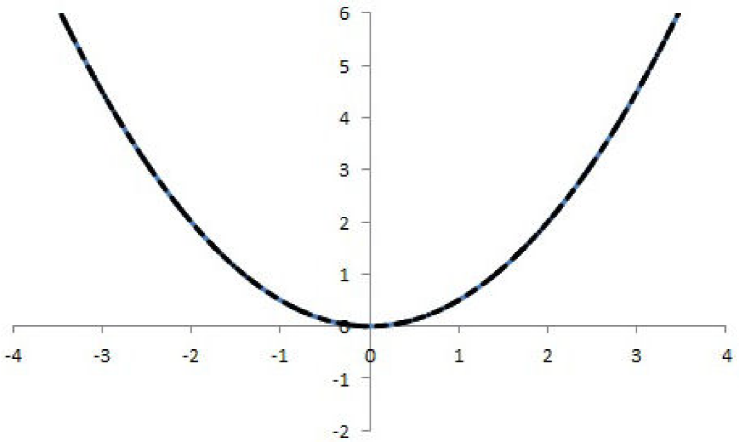
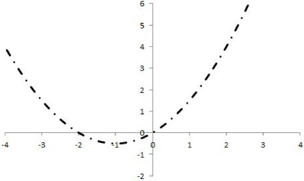
Figure 4. The potential for α=0. It represents the harmonic oscillator potential in the presence of an electric field. 

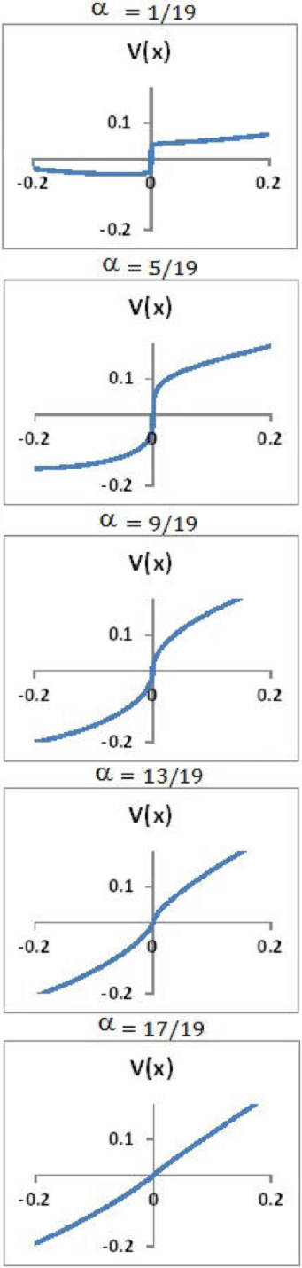
Figure 5. The potential for selected values of α. The figure shows the evolution process of the potential which affects the wave function. 

It is worth mentioning that the shifts should reverse directions if the electric field is applied in the opposite direction, or considering a negative charge.

4. Conclusion

We demonstrate the effect of an evolved electric potential on a charged particle placed in a harmonic oscillator. The effect of the evolved potential on the wave function and energy is shown for different states, where the wave function experienced a shift towards increasing fraction. We also show how the potential itself develops fractionally and how it was reshaped until it takes the form a fully developed potential. In future work, the anharmonic oscillator will be studied fractionally to have a better understanding of thermal expansion.

References

1. N. Laskin, Phys. Lett. A. 268 (2000) 298-305. [ Links ]
2. J. Dong, M. Xu, J. Math. Anal. Appl. 344 (2008) 1005-1017. [ Links ]
3. D. Jianping, Eprint ArXiv13013009. (2013). [ Links ]
4. B.N. Narahari Achar, J.W. Hanneken, T.J. Clarke, J.M. Skaggs American Physical Society March meeting (2000). [ Links ]
5. P. Rozmej, B. Bandrowski, Comput. Methods Sci. Technol. 16 (2010) 191. [ Links ]
6. Avik Kumar Mahata. Int. J. Sci. Eng. Res. 4 (2013). [ Links ]
7. R. Herrmann arXiv: 1210.4410v2 [math-ph] (2012). [ Links ]
8. R.W. Ibrahim, H.A. Jalab J. Inequalities Appl. 23 (2015). [ Links ]
9. N. Laskin, Phys. Rev. E. 66 (2002) 056108. [ Links ]
10. N. Laskin, Phys. Rev. E. 62 (2000) 3135. [ Links ]
11. X. Guo, M. Xu, J. Math. Phys. 47 (2006) 082104. [ Links ]
12. R. Herrmann, Fractional calculus: an introduction for physicists. Hackensack, NJ: World Scientific. 479 pp. 2nd edition ed. (2014). [ Links ]
13. A. A. Kilbas, H.M. Srivastava, J.J. Trujillo, Theory and applications of fractional differential equations Amsterdam; Boston: Elsevier. 523 pp. 1st ed. (2006). [ Links ]
14. I. Podlubny, Fractional differential equations: an introduction to fractional derivatives, fractional differential equations, to methods of their solution and some of their applications. San Diego: Academic Press. 340 pp. (1999). [ Links ]
15. N. Engheta, IEEE Trans. Antennas Propag. 44 (1996) 554. [ Links ]
16. N. Engheta, Microw. Opt. Technol. Lett. 23 (1999) 100. [ Links ]
17. D.H. Werner, R. Mittra, In Frontiers in Electromagnetics, IEEE. 1st ed. (2000) p. 523. [ Links ]
18. A. Rousan, E. Malkawi, E. Rabei, H. Widyan, Fract. Calc. Appl. Anal. 5 (2002) 155. [ Links ]
19. A. Rousan et al. Fract. Calc. Appl. Anal. 9 (2006) 33. [ Links ]
20. A. Rousan N. Ayoub K. Khasawineh, Int. J. Apllied Math. 19 (2006) 263. [ Links ]
21. J.F. Gómez-Aguilar, Rev. Mex. Fís. 62 (2016) 144. [ Links ]
22. J.F. Gómez-Aguilar, R. Razo-Hernandez, D. Granados-Lieberman, Rev. Mex. Fís. 60 (2014) 32-38. [ Links ]
23. F. Gómez, J. Rosales, & M. Guia, Central European Journal of Physics, 11 (2013) 1361-1365. [ Links ]
24. Guia, M., Gómez, F., & Rosales, J. Open Physics, 11 (2013) 1366-1371. [ Links ]
25. J.F. Gómez-Aguila & E. Alvarado-Méndez, (2015) (pp. 147-158) Springer Netherlands. [ Links ]
26. J.F. Gómez-Aguilar, H. Yépez-Martinez, C. Calderón-Ramón, M. Benavidez-Cruz, & L.J. Morales-Mendoza, Journal of Electromagnetic Waves and Applications (2015) 1-13. [ Links ]
27. T. Kaczorek, & K. Rogowski, Springer International Publishing. (2015) (pp. 81-115). [ Links ]
28. T. Kaczorek , & K. Rogowski, (2015) Springer International Publishing (pp. 49-80). [ Links ]
29. A. Obeidat, M. Gharaibeh, M. Al-Ali, A. Rousan, Fract. Calc. Appl. Anal. 14 (2011) 247. [ Links ]
30. S. Gasiorowicz, Quantum physics. 336 (2003) 3. [ Links ]
31. M.M. Chawla, BIT Numerical Mathematics 24 (1984) 117-8. [ Links ]
32. C.P. Katti, K. Chopra, International Journal of Computer Mathematics 37 (1990) 221-6. [ Links ]
33. R. Gonsalves Phy410-505-2009. Computational Physics. https://www.physics.buffalo.edu/phy410-505-2009/. (2009). [ Links ]
Received: May 02, 2016; Accepted: June 03, 2016
Creative Commons License This is an open-access article distributed under the terms of the Creative Commons Attribution License