1. Introduction

From the earliest days of quantum mechanics, it has been clear that one could not hope to solve most of the physically interesting systems exactly, especially those with more particles. Thus, by 1930 (only three years after the first works of Thomas¹ and Fermi², and five years after the advent of the “new” quantum theory), a large variety of approximate methods had been developed to construct approximate analytical solutions for nonlinear differential equations. There has been a great deal of work on rigorous mathematical problems in quantum theory, most of it on the fundamentals and relevant operator theory.

The Thomas-Fermi equation is a nonlinear ordinary differential equation for modeling electrons of an atom. In particular, the Thomas-Fermi model is widely used in nuclear physics, for example, to answer questions related to nuclear matter in neutron stars³. In spite of its generality, the application of the Thomas-Fermi method is based on the solution u(x) of the second-order nonlinear differential equation which is difficult to determine.

The purpose of this model is give a expression for the electron density 𝜌(𝑟), and of course, the electrostatic potential between the nucleus and the cloud of electrons at a distance 𝑟 for this. This central potential 𝑉(𝑟) dominates the interaction of electrons obeying Fermi-Dirac statistics in a volume region considered to be large that does not vary appreciably over the size of the region. In this case the electrons move freely. In this conditions, the electron kinetic energy is a minimum, and the electrons are packed in phase space as densely as possible consistent with the exclusion principle. If 𝑝 max is the maximum value for the electron momentum

where 𝑛 is the number of electrons per unit volume. The potential energy is −𝑒𝑉, and it is confined in a neutral atom if its energy is non-positive, i.e.

Using the expression (2) into (1), we can express the electron charge density in terms of the potential 𝑉,

Now the electronic charge density 𝜌(𝑟) and the potential 𝑉(𝑟) are related via the Poisson equation:

Taking into account the solution of (4), the boundary conditions are such that 𝑉(𝑟) tends to 𝑍𝑒/𝑟 when 𝑟→0 (Coulomb field), and 𝑉(𝑟) tends to zero when 𝑟 tends to infinity.

The Thomas-Fermi equation in its usual form is presented when performing a change of variable

where 𝑎 0 =( ℎ 2 /4 𝜋 2 𝑚 𝑒 𝑒 2 )=5.2917721092 .10 −11 𝑚≈0.53 Å, is the first Bohr radius of the hydrogen atom, at a distance 𝑟 from the nucleus, 𝑚 𝑒 and 𝑒 are the mass and charge of electron.

This change is also convenient because it eliminates all numerical constants in Eq. (4) leading to an universal nonlinear second-order ordinary differential equation which describes all atoms without distinguishing their composition or number of electrons. Substituting the changes described in ([change]) into Eq. ([poisson]), we find the Thomas-Fermi equation

This new Eq. (6) satisfies

An important parameter is the magnitude of the initial slope

such as under numerical integration yields 𝐵=0.5055 𝜋=−1.588⁴.

There have been many attempts to construct an approximate analytical solution of the Thomas-Fermi equation for atoms⁵. E. Roberts⁶, in these cases using variational principles, trying to solve the equation by proposing a one-parameter trial function:

where 𝜂=1.905 and Csavinsky⁷ has proposed a two-parameters trial function:

where 𝑎 0 =0.7218337, 𝛼 0 =0.1782559, 𝑏 0 =0.2781663 and 𝛽 0 =1.759339. Later, Kesarwani and Varshni⁸ suggested:

where 𝑎=0.52495, 𝛼=0.12062, 𝑏=0.43505,𝛽=0.84795, 𝑐=0.04 and 𝛾=6.7469.

The last two equations are obtained using an equivalent Firsov’s variational principle⁹. The first equation has been modified by Wu in the following form:

where 𝑚=1.14837 and 𝑛=4.0187⋅ 10 −6 .

Recently, M. Desaix et al. proposed the following expression:

where 𝑎=0.9237797117, 𝑏=2.097976638 and 𝑘=0.4834685937. Moreover, other attempts have been carried out to solve this problem^12),(13. But, all of these proposed trial functions do not reproduce appropriately the numerical solution of the Thomas-Fermi equation¹⁴ and its derivative at 𝑥=0. They did not prove to be efficient when used to calculate the total ionization energy of heavy atoms.

Oulne¹⁵, proposed a trial function which depends on three parameters 𝛼, 𝛽 and 𝛾:

The optimum values of the variational parameters 𝛼, 𝛽 and 𝛾, obtained by minimizing the Lagrangian, are respectively equal to 0.7280642371, -0.5430794693 and 0.3612163121.

From other methods Marinca et al.¹⁶, solve the Thomas-Fermi equation in this case using OHAM (Optimal Homotopy Asymptotic Method), finding a pair of approximate solutions with good accuracy. These solutions are somewhat complicated, introducing many parameters in a combination (or rather a generalization) of solutions found previously for other authors by simpler functions. Bougoffa et al¹⁷ work with a new technique for solving the Thomas-Fermi equation. They first reduce it to an equivalent second-order differential equation, and then they express the solution in the logarithmic form to obtain a good approximate solution in a straightforward manner by using a direct approach.

The purpose of this manuscript is give a solution to Thomas-Fermi equation with a modified trial solution of Wu’s function depending on three parameters and satisfying the boundary conditions. The found solution is used to calculate the total ionization energy of atoms, taking into account a correction to this equation. Our results show that the proposed generalization is much better than Wu’s one, being in agreement with other solutions found in literature and reproducing conveniently the corresponding numerical solution.

2. Variational approach for Thomas-Fermi equation and a correction of ionization energies

We use variational techniques and optimization to find analytical solutions. In this case, the idea is that the Thomas-Fermi differential equation can be described by the following Lagrangian

this Lagrangian is equivalent to Eq. ([tf]), when one use the Euler-Lagrange equation

where the prime symbol denotes derivative respect to 𝑥 variable. Finally, the total Lagrangian is constructed in the form

thus when a solution is fixed, 𝑢=𝑢(𝑥, 𝛼 𝑖 ), 𝑖=1,2,3..., in terms of some coefficients, then it can be optimized using a total Lagrangian minimum condition to find the value of arbitrary constant

There has been a considerable renewed interest in calculating leading corrections, to the binding energy of the Thomas-Fermi atom. The problem of incorporating the first leading correction in the Thomas-Fermi model was predicted by Scott¹⁸, the values for the second and the third corrections were suggested by Marchand Paskett¹⁹ and Schwinger⁴. Taland Levy²⁰ suggested that a 𝑍 −1 expansion could lead to a better fit for the total binding energy of the Thomas-Fermi atom. In this way, ²¹uses the 𝑍 −1 expansion to re-write the ionization energy of a many-electrons atom to the second leading corrections, in terms of the initial slope of the trial variational solutions of the Thomas-Fermi equation, where no attention has been paid to the calculation of these nonzero order corrections in terms of trial variational functions of the variational schemes which replaces the Thomas-Fermi theory.

A test to demonstrate the efficiency of the different solutions can be made by calculating the total ionization energy of heavy atoms following the relation²²

in hartrees ( 𝑒 2 / 𝑎 0 ). This expression can be considered as a zero-order correction of the total binding energy. The first derivative of 𝑢′(𝑥) evaluated in the origin, is the initial scope of 𝑢(𝑥). Numerical calculations give a value 𝑢′(0)=−𝐵 =−1.588070972, also called Baker’s constant. For the leading corrections, Agil et al. give a correction for Eq. (19). They used a technique in which the correction becomes a expansion over 𝑍 −1 , and applied it to the Thomas-Fermi model. The corrected second order equation found is

where

and

As can be easily seen the resulting Eq. (20) for the binding energy reduces to the zero-order Thomas-Fermi energy for 𝑢′(0)=−𝐵, and 𝐹(𝑍)→1 corresponding to large atomic numbers. In general, this model could be applied to various possible suitable trial functions.

3. Results

In the present paper, we suggest the following modified variational trial solution of Wu’s function for the Thomas-Fermi equation adding a new parameter:

In this case, the total Lagrangian (17), is a bit more complicated but can be simplified as 𝐿 𝑡 = 𝐿 1𝑡 + 𝐿 2𝑡 , where

and

Then, when we minimize the Lagrangian through (18), we found the values of parameters in the trial solution:𝑎=0.9614236887819619, 𝑏=−0.3442527917822383 and 𝑐=0.08703140640977791.

The values of the functions proposed by Wu, our solution, and Oulne’s solutions are shown in the Table 1. We can see that all functions satisfy the boundary conditions (7), obtaining accurate results. In Table 1, the relative error (%) of the solutions is shown in comparison to the numerical solution¹⁴.

In the Table 2, we present the ionized energies calculated for all solutions, and compared them with the Hartree-Fock (HF) numerical solution²³. In the last row, we show the average error is obtained from all 16 tested points, 2≤𝑍≤86.

4. Conclusions

We have proposed a trial function that generalizes Wu’s proposal function making use of variational techniques to solve the Thomas-Fermi differential equation. Comparing the results in Table I, we can see that the Eq. (23) has a lower error compared with Wu’s corresponding solution throughout the measured range. The average error calculated for Wu’s solutions is 25.12% for Eq. (12), compared with the error found for our solution which is 4.86% taking into account 67 points for the 𝑥 values.

Furthermore, in the test of efficiency for various heavy atoms, we can see that our errors are smaller compared with

Table 1 The values of the functions proposed by Wu, our solution, Oulne’s solutions, and the corresponding comparison of the relative error (%) of the functions respect to the numerical solutions. In this case Er(uNum; uk) = (uNum ¡ uk=uNum)£100. In the last row, the average or error is obtained based in 67 points of values of x and is defined (1=n) Pni=1(uNum ¡ uk=uNum)100. 

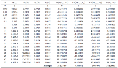
Table 2 Comparison of total ionization energies E in units (e2=a0) from HF and the found solution. In the last row, the average or error is taken for the values of Z and is defined (1=n) Pn i=1(juNum ¡ ukj=uNum)100. 

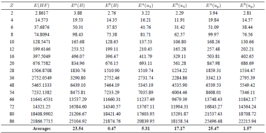
a Values corresponding to energy uncorrected calculated mean Eq. (19).

b Values corresponding to energy corrected calculated with the correction mean Eq. (20).

E(B) Correspond to energy for numerical result, u0(0) = ¡B = ¡1:588070972.

the solutions found by Wu. However, we can also see that the correction from ionization energies using (20) not only reproduce better the energies calculated numerically by HF, but also produce a better approximation with our solution. However, we also notice that the energy calculation using the uncorrected equation is better for Wu’s solution compared to ours, contrary to what occurs with the equation suggested by²¹.

The derivative of our function (23) at 𝑥=0 is equal to -1.61284 just as for our function (14), which is closer to the numerical derivative: -1.58807102¹⁴ compared with the derivative of function (12) at 𝑥=0 which equals to -1.31828.

As we can see our results are accurate without the need to appeal to the resolution of subsidiary conditions, in contrast to most of variational solutions found years ago in the literature. Each integral has been solved analytically without the use of corresponding numerical methods.