


 text new page (beta)
 English (pdf)
 Article in xml format
 Article references
 Send this article by e-mail
 Cited by SciELO
  Similars in
SciELO
Similars in
SciELO 
 Permalink
PACS: 40.05.+e; 47.10.ab; 47.15.Cb; 47.50.-d; 47.56.+r
1. Introduction
It is well known phenomena that traditional Newtonian fluid is inadequate to describe the characteristics of fluid with suspended particles. The non-Newtonian fluid that incorporates the motion of suspended particles is the micropolar fluid. Micropolar fluids consist of randomly oriented dumb-bell shaped particles that can undergo a rotation. Some examples of such fluids are colloidal fluids, biological fluids, polymeric fluids, liquid crystal and exotic lubricants etc. The rotation of these particles affects the overall dynamics of the flow phenomena. Eringen 1 first derived the governing equations of micropolar fluids and later extended it to the theory of thermomicropolar fluids 2. In flow equations describing micropolar fluid phenomena, the principle of conservation of angular momentum is essential along with the standard equations for the conservation of mass and momentum. The details regarding the theory of micropolar fluids can be seen in the book by Lukaszewics 3. The theory of micropolar viscoelastic is established for such problems in which the typical theory of viscoelastic is unavailable due to microstructure in the substance. Generally, these problems are related to grain bodies and multimolecular materials like polymer. Eringen4 constructed the linear theory of microplar viscoelasticity. McCarthy and Eringen 5 studied the propagation of waves in micropolar viscoelastic medium. Saint-Venant’s principle of micropolar viscoelastic substances was described by DeCicco and Nappa 6. Kumar 7 presented the wave propagation in micropolar viscoelastic generalized thermoelastic solid. For application point of view, one can study Kumar and Choudhary 8 in which they investigated the dynamic problem in micropolar viscoelastic medium.
Diffusion of chemically reactive species into the fluid from the surface is another important area of research in recent years. The applications of such process include polymer production, manufacture of ceramics and glassware, food processing etc. Chambre and Young 9 investigated the diffusion of chemical reactive species in a laminar boundary layer flow. The problem discussed in Ref. 9 was extended for a stretching sheet by Anderson et al. 10. Mohamed and Abo-Dahab 11 investigated the influence of chemical reaction and thermal radiation in a MHD micropolar fluid. They also incorporated the effects of porous medium. The effect of MHD, mass transfer and chemical reaction in a second grade fluid flowing through a porous medium over a stretching sheet was discussed by Cortell 12. In another paper, Cortell 13 presented the numerical solution for two classes of viscoelastic fluids with chemically reacting species. A literature survey reveals that different aspects of flow have been investigated under the diffusion of chemically reactive species. Das et al. 14 presented the effects of homogeneous first order chemical reaction on the flow past an impulsively started plate. Muthucumaraswamy 15,16 respectively investigated the influence of chemical reaction on the flow past an impulsively started vertical plate with uniform heat and mass flux without and with suction. The problem of wedge flow with suction and injection and chemical reaction has been considered by Devi and Kandasamy 17. The further details of influence of chemically reacting species on different flow situations can be seen in the literature 18-25. Stagnation point flow of viscoelastic fluid has been investigated by Beard and Walters 26. They have obtained a perturbation solution of problem up to first order. The problem of stagnation point flow in a micropolar fluid was studied by Nazar et al. 27. A literature survey reveals that stagnation point flow has been investigated for a range of non-Newtonian fluids, for example see Xu et al. 28, Hayat et al. 29, Abbas et al. 30, Sajid et al. 31, Yacob et al.32, Hayat et al.33, Mosta et al. 34, Nandy 35 and many references there in. In a study El-Kabir 36 combined the effects of micropolar and viscoelastic fluids and discussed the hydromagnetic stagnation point flow in a micropolar viscoelastic fluid. In a recent paper Abbas et al. 37 discussed the heat transfer analysis in a micropolar viscoelastic fluid past a stretching/shrinking sheet in the presence of magnetic field.
The objective of the present paper is to study the stagnation point flow of micropolar viscoelastic fluid past a stretching/shrinking sheet immersed in a porous medium with chemically reactive species. In this problem for viscoelastic fluid, we considered the Walters’ B model. The problem is formulated using nth-order homogeneous chemical reaction of constant rate k n . With the help of suitable transformations the governing partial differential equations are converted to ordinary differential equations and then solved analytically using homotopy analysis method.
2. Formulation of the problem
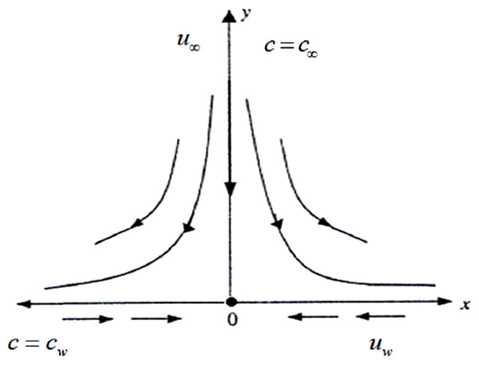
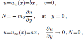
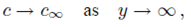
Consider a steady, incompressible and two-dimensional stagnation-point flow of a micropolar viscoelastic fluid embedded in a porous medium due to a stretching/shrinking surface at y=0 the flow covers the region y>0. The sheet is stretched/shrunk in the x- direction so that the x-component of velocity is u w (x)=bx where b>0 and b<0 are for stretching and shrinking cases, respectively. It is also assumed that the velocity of the external flow is given by u ∞ (x)=ax, where a>0 is the strength of the stagnation flow. By assuming c w and c ∞ . As the concentrations at the wall and far away from the sheet, respectively, mass transfer analysis is also carried out. Following Eringen 4, El-Kabeir 36 and Muhaimin et al. 38, the basic governing boundary layer equations of micropolar viscoelastic fluid and concentration field in the absence of body forces are:
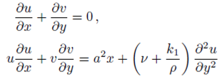 (1)
(1)
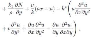 (2)
(2)
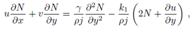 (3)
(3)
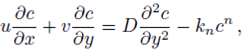 (4)
(4)
here u and v are the velocity components in the x- and y-axis directions, respectively, v is the fluid kinematic viscosity, k 1 is the vortex viscosity, ρ is the fluid density, N is the micro-rotation or angular velocity, k is the permeability of the porous medium, k* is the Weissenberg number, γ is the spin gradient viscosity and j is the microinertia per unit mass, whereas c is the concentration of the fluid, D is the diffusion coefficient and k n is the n th-order chemical reaction rate constant.
It is clear from Eq. (2) that the order of partial differential equation is higher than the Navier-Stokes equations. Therefore, one needs an additional boundary condition. Garg and Rajagopal 39 proposed the idea of augmenting the boundary condition at the free stream.
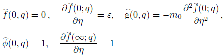
Implementing the same here, we have the following boundary conditions for the present flow:
 (5)
(5)
 (6)
(6)
where ‘a’ and ‘b’ both are constant having dimension (time)-1 and m 0 (0 ≤ m 0 ≤ 1) is a constant. Whereas, m 0 =0 represents that the concentrated particle flow where the microelements near the wall surface are not able to rotate (i.e.N=0). This situation is called strong concentration of microelements 40. However, m 0 =1/2 implies the vanishing of anti-symmetric part of the stress tensor and known as weak concentration of microelements 41. Here in this problem we just take into account the case of m 0 =0.
We use the following non-dimensionalize variables to simplify the flow problem
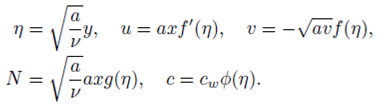 (7)
(7)
With the help of Eq. (7), the continuity Eq. (1) is identically satisfied and Eqs. (2-4) take the form
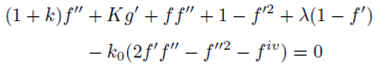 (8)
(8)
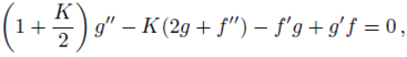 (9)
(9)
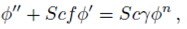 (10)
(10)
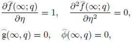
subject to the boundary conditions
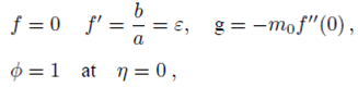 (11)
(11)
 (12)
(12)
where a prime is a differentiation with respect to η, k=k
1
/pv is the micropolar parameter, k
0
=ak*/vp is the viscoelastic parameter, λ=v/ka is the porosity parameter, Sc=v/D is the Schmidt number,
It is evident from Eq. (13) that the highest derivative term has a coefficient k 0 ƒ which is zero at η=0 and when k 0 →0 i.e. for a viscous micropolar fluid. Therefore, due to singularity at the starting point of the domain the numerical solution is not straight forward.
The wall shear stress is defined as
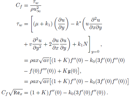 (13)
(13)
The wall couple stress is defined as
in which G=G 1 a/v is the microrotation parameter and G 1 =γ/k 1 is the microrotation constant.
The Sherwood number is defined as
Where Re x =ax 2 /v is a local Reynolds number.
3. Homotopy analysis solution
Homotopy analysis method is used to get the series solutions of the non-linear boundary value problems consisting of Eqs. (8)-(10) with boundary conditions (11) and (12). The set of base functions for fluid velocity ƒ(n) angular velocity g(η) and concentration field ɸ(η)can be defined as
in the form
here
and the auxiliary linear operators
that satisfy the following properties
Where C i (i=1,2,3,4,5,6,7) are arbitrary constants, which can be determined using boundary conditions (11) and (12).
The zeroth-order deformation problems are constructed as follows:
 (29)
(29)
 (30)
(30)
 (31)
(31)
 (32)
(32)
 (33)
(33)
where q∈[0,1] is an embedding parameter and ћ ƒ, ћ g and ћ Φ denote the non-zero auxiliary parameters, the non-linear operators N ƒ , N g and N Φ are
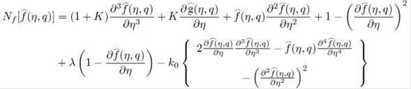 (34)
(34)
 (35)
(35)
 (36)
(36)
The above zeroth- order Eqs. (29)-(31) possess following solutions for q=0 and q=1
By using Taylor’s series with regard to q we get
here
For the convergence of the series solutions, the values of ћ ƒ, ћ g and ћ Φ are selected in such a way that at q=1 the given series are convergent and finally the series solutions are of the form:
For m th-order deformation equations, we simply differentiate the zeroth-order deformations Eqs. (29)-(31), m times with respect to embedding parameter then take q=0 and finally dividing by m! then we have
 (49)
(49)
where
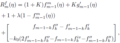 (52)
(52)
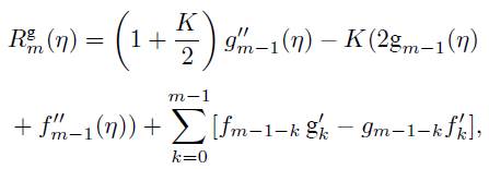 (53)
(53)
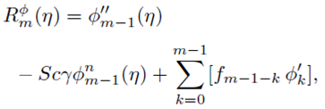 (54)
(54)
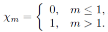 (55)
(55)
Let
in which the values of constants C i (i=1,2,3,4,5,6,7) are achieved through boundary conditions (50) to (51) as
Using software Mathematica or any other, one might solve Eqs. (47)-(49) one after the other in the order m=1,2,3,4…
4. Convergence of HAM solution
By applying homotopy analysis method, the analytical solutions in the form of series must converge to the exact solution of original problem which is under consideration and it is already explained by Liao 43. Many researchers 44-52 applied this method to solve highly non-linear problems. To ensure the convergence region and rate of approximation for the homotopy analysis method, the non-zero auxiliary parameters ћ
ƒ, ћ
g and ћ
Φ
are chosen accurately by plotting the so-called ћ-curves. In Figs. 2a and 2b, the ћ-curves of ƒ’’(0) , g’(0) and Φ’(0) at 20th-order of approximation are shown. It is noted from these figures that
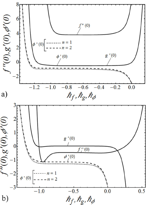
FIGURE 2 a) The ħ -curves of ƒ’’ (0), g’(0) and Φ’ (0) at 20th-order of approximation for k 0 = 0.5, K = 0.5, λ = 0.5, β = 3, S c = 1 and γ = 1 in the case of shrinking sheet. b) The ħ curves of ƒ’’ (0), g’(0) and Φ’ (0) at 20th-order of approximation for k 0 = 0.5, K = 0.5, λ = 0.25, β = 3, Sc = 1 and γ = 1 in the case of stretching sheet.
5. Results and discussion
The non-linear boundary value problem consisting of Eqs.(8)-(10) with boundary conditions (11) and (12) is solved analytically by means of homotopy analysis method in the whole domain (0 ≤ η ≤ ∞) to compute the fluid velocity ƒ’(η), microrotation or angular velocity g(η) and the concentration field Φ(η). The fluid velocity component, angular velocity and the concentration profiles are plotted to observe the effects of the various involving parameters, for example the micropolar parameter K, porosity parameter λ, viscoelastic parameter k 0 , Schmidt number Sc and chemical reaction rate parameter γ in Figs. (3)-(12). Furthermore, we have computed and showed the numerical values of the skin-friction coefficient, wall couple stress and the Sherwood number for several physical parameters both graphically and in tabular form. The comparison of the present results with the existing results is given in limited cases, and we found them to be in excellent agreement.
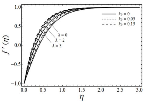
FIGURE 3 Velocity profiles for various values of the porosity parameter λ and the viscoelastic parameter K with micropolar parameter K 0 = 0 and β = 3 in case of shrinking sheet.
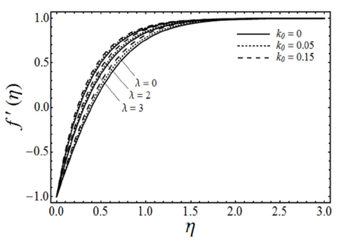
FIGURE 4 Velocity profiles for various values of the porosity pa- rameter λ and the micropolar parameter K with viscoelastic pa- rameter k0 = 0.5 and β = 3 in case of shrinking sheet.
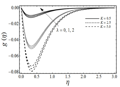
FIGURE 5 Microrotation profiles for various values of the poros- ity parameter λ and the micropolar parameter K with viscoelastic parameter k 0 = 0.5 and β = 3 in case of shrinking sheet.
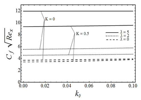
FIGURE 6 Variation of skin friction coefficient with the viscoelas- tic parameter k 0, for various values of micropolar parameter K and the porosity parameter λ with β = 3 in case of ε = −1.
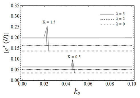
FIGURE 7 Variation of |g t (0)|, which is proportional to the wall couple stress, with the viscoelastic parameter k0, for various values of the micropolar parameter K and the porosity parameter λ with β = 3 in case of ε = −1.
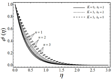
FIGURE 8 Concentration profiles for various values of the microp- olar parameter K and the viscoelastic parameter k 0 with porosity parameter λ = 1 Schmidt number Sc = 2, chemical reaction rate parameter γ = 2 and β = 3 in case of shrinking sheet.
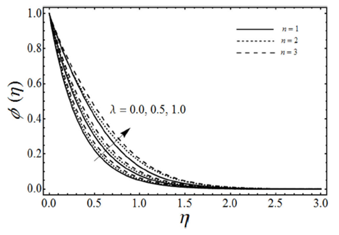
FIGURE 9 Concentration profiles for various values of porosity parameter λ with micropolar parameter K = 3, viscoelastic parameter k 0 = 2, Schmidt number Sc = 2, chemical reaction rate parameter γ = 2 and β = 3 in case of shrinking sheet.
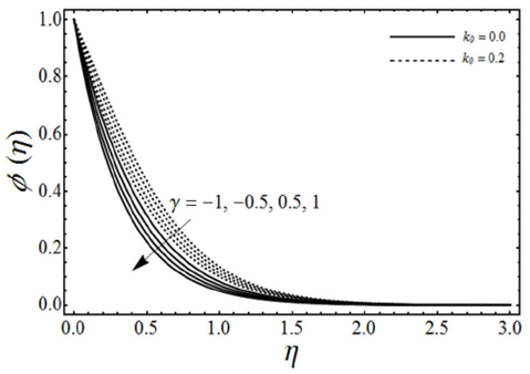
FIGURE 10 Concentration profiles for various values of the chemical reaction rate parameter γ and the viscoelastic parameter k 0 with porosity parameter λ = 1, micropolar parameter k = 0.5, Schmidt number Sc = 2, β = 3 and n = 2 in case of shrinking sheet.
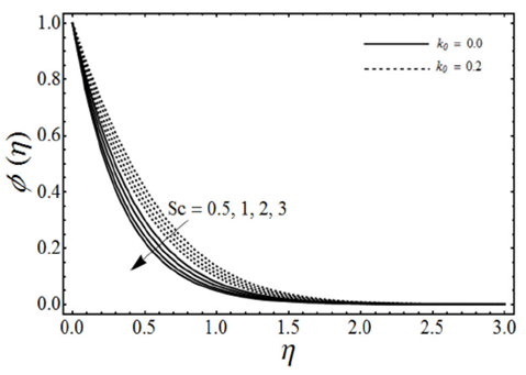
FIGURE 11 Concentration profiles for various values of the Schmidt number Sc and the viscoelastic parameter k 0 with porosity parameter λ = 1, micropolar parameter K = 0.5, chemical reaction rate parameter γ = 2, β = 3 and n = 2 in case of shrinking sheet.
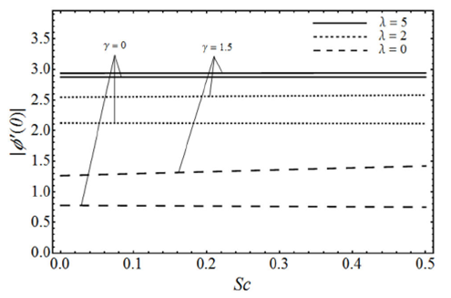
FIGURE 12 Variation of | Φ’ (0)|, for various values of the Schmidt number Sc and porosity parameter λ with the viscoelastic parameter k 0 = 0.5, the micropolar parameter K = 0.5 and β = 3 in case of ε = −1.
Figure 3 shows the variation in the fluid velocity component ƒ’(η) for several values of a viscoelastic parameter k
0
and porosity parameter λ in the case of (K=0) with β and ɛ fixed. From this Fig. 4, it is evident that the fluid velocity ƒ’(η) increases with an increase in both λ and k
0
. Figure 4 gives the change in the fluid velocity component ƒ’(η) for various values of the porosity parameter λ and the micropolar parameter K (in the case of viscoelastic fluid k
0
=0.5) by keeping β and ɛ fixed. It is found in figure that the fluid velocity increases with an increase in porosity parameter λ by keeping the values of K constant, but on the other side as we increase the values of micropolar parameter K the fluid velocity ƒ’(η) decreases. However with the increasing values of micropolar parameter K the momentum boundary layer thickness increases. Figure 5 elucidates the effects of the porosity parameter λ and the micropolar parameter K on the angular velocity g(η) in case of viscoelastic fluid (k
0
=0.5) with other parameters β and ɛ are fixed. From this figure we can see that the angular or microrotation velocity g-(η) goes to decrease by increasing the values of micropolar parameter K whereas it increases with an increase in porosity parameter λ. It is also noted from this figure that the angular velocity over shoot near the sheet due to a microrotation of the fluid particles. Figure 6 gives the variation of the skin-friction coefficient
The change in the concentration field Φ(η) for different values of homogeneous chemical reaction rate n, viscoelastic parameter k 0 and micropolar parameter K in the case of destructive chemical reaction γ=2 is presented in Fig. 8 keeping β and ɛ fixed. From this figure we can see that the concentration field Φ(η) is increased with an increase in n and K, whereas it decreases by increasing the values of viscoelastic parameter k 0 . Figure 9 shows the influence of the concentration field Φ(η) for several values of porosity parameter λ and n in the case of destructive chemical reaction (γ=2) by keeping K, k 0, S c , β and ε fixed. It is observed from this figure that the concentration field is increased with an in-crease in both n and λ. Figure 10 gives the variation of the concentration field Φ(η) for various values of the generative/destructive chemical reaction parameter γ and viscoelastic parameter k 0 with λ, K, k 0 , Sc, n, β and ɛ are fixed. It can be seen from this figure that as γ increases from -1 to 1, we can find the decrease in the concentration field Φ(η), whereas the concentration field increases with an increase in viscoelastic parameter k 0 . Figure 11 describes the behaviour of the concentration field Φ(η) for several values of the Schmidt number Sc and viscoelastic parameter k 0 in the case of destructive chemical reaction parameter (γ=2 by keeping λ, K, n, β and ɛ fixed. From this figure we can see that with the increasing values of Sc dimensionless concentration field Φ(η) decreases while it increases by increasing the values of viscoelastic parameter k 0 . Figure 12 depicts the variation of the Sherwood number or the rate of mass transfer at the wall | Φ’(0)| versus the Schmidt number Sc for various values of the porosity parameter λ and the chemical reaction parameter γ by keeping K, k 0 , n, β and ɛ fixed. From this figure it is evident that the magnitude of the Sherwood number is increased with an increase in both γ and λ.
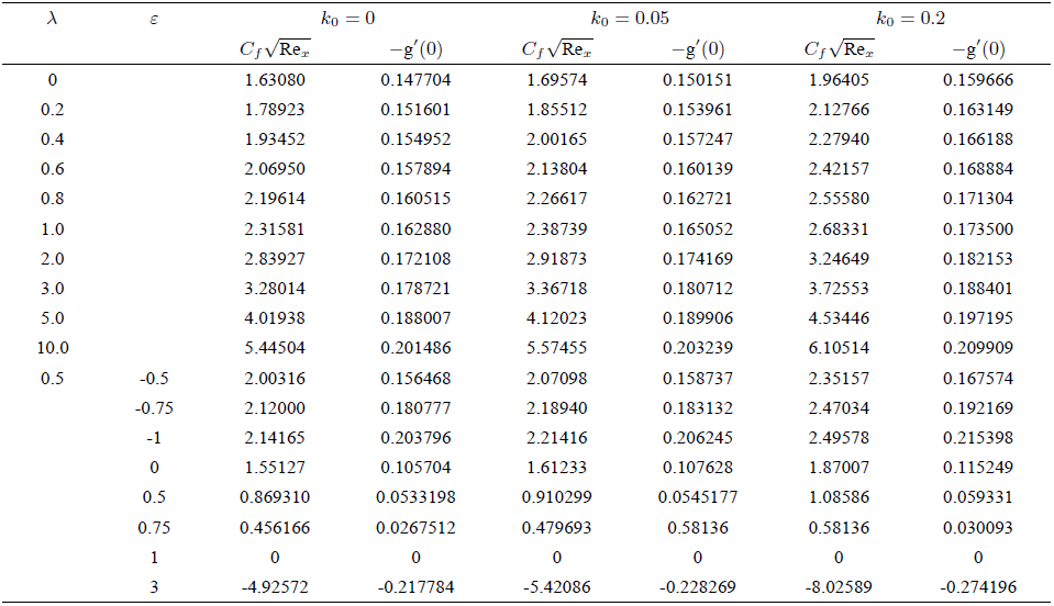
Table II is made to show the numerical values of the skin-friction coefficient
TABLE II Comparison of present results of wall shear stress
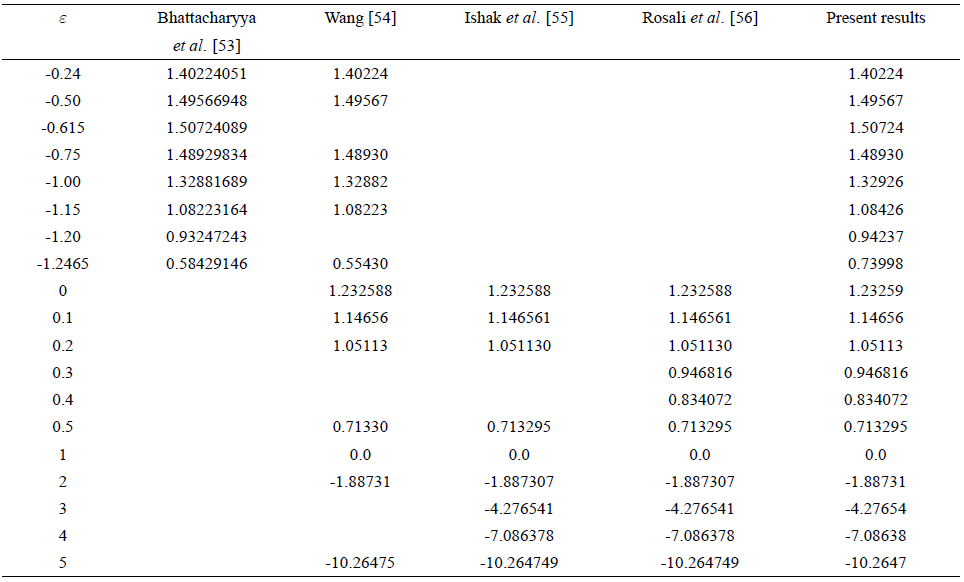
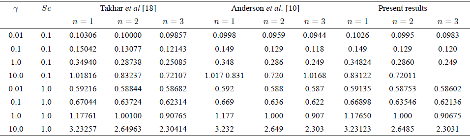
TABLE III Comparison of present results of Sherwood number with the existing results in the case of Newtonian fluid for stretching sheet.
6. Concluding remarks
The two-dimensional stagnation point flow of an electrically conducing micropolar viscoelastic fluid in a porous medium over a stretching/shrinking sheet in the presence of chemical reaction is investigated in this paper. The similarity transformations are used to convert the partial differential equations to a set of ordinary differential equations, and hence a analytical solution is obtained using homotopy analysis method. The fluid velocity, angular velocity and concentration profiles as well as local skin-friction coefficient, local wall couple stress and local Sherwood number are shown graphically and analyzed for various physical parameters of interest. From this study, we have made the following observations:
The fluid velocity and angular velocity profiles are increased by increasing k 0 and λ whereas both are decreased with an increase in K.
The skin-friction coefficient and wall couple stress increase by increasing K, k 0, and λ.
It can also be concluded that the presence of Schmidt number and chemical reaction parameter is to decrease the concentration field whereas the presence of porosity parameter and rate of homogenous chemical reaction constant increases the concentration field.
It is also observed that the presence of chemical reaction, Schmidt number and porosity medium is to increase the Sherwood number.

