


 nueva página del texto (beta)
 Inglés (pdf)
 Artículo en XML
 Referencias del artículo
 Enviar artículo por email
 Citado por SciELO
  Similares en
SciELO
Similares en
SciELO 
 Permalink
PACS: 02.30.Hq; 03.65.Fd; 04.20.Jb
1.- Introduction
Fractional differential equations are generalizations of classical differential equations of integer order. In recent years, nonlinear fractional differential equations (NFDEs) have gained considerable interest. It is caused by the development of the theory of fractional calculus itself but also by their applications in various sciences such in physics, biology, engineering, signal processing, system identification, control theory, finance and fractional dynamics and others areas 1-9. A special class of analytical solutions, the so-called traveling waves for nonlinear fractional partial differential equations (NFPDEs), is of fundamental importance because several physical models are often described by such wave phenomena. However, not all NFPDEs are solvable. As a result, recently new techniques have been successfully developed to construct new solutions for fractional nonlinear partial differential equations of physical interest, such as the Adomian decomposition method 10-11, the variational iteration method (14-15), the homotopy analysis method 12-13, the homotopy perturbation method 16-17, the Lagrange characteristic method 16-17, the fractional sub-equation method19, and so on.
In Ref. 20, Jumarie proposed a modified Riemann-Liouville derivative. With this kind of fractional derivative and some useful formulas, we can convert fractional differential equations into integer-order differential equations by variable transformation.
Feng 21 has introduced a reliable and effective method called the Feng’s first integral method to look for traveling wave solutions of NFPDEs. The basic idea of this method is to construct a first integral with polynomial coefficients by using the division theorem. This method in comparison with other methods has many advantages; it avoids a great deal of complicated and tedious calculation and provides exact and explicit traveling solutions with high accuracy. The Feng’s first integral method 22-25 can be used to construct the exact solutions for some time fractional differential equations.
Among the nonlinear PDEs there are some important examples of fundamental interest in mathematical-physical models. For example, some types of coupled Korteweg de-Vries (KdV). The coupled KdV equation describes, in a general form, competition between the weak nonlinearity and the weak dispersion in many physical systems. Since the first coupled KdV system was presented by Hirota and Satsuma in 1981 26 and have been carefully studied in Refs. 27 and28. Some important coupled KdV models have been proposed 29-30. In Ref. 31 the authors have introduced a 4 × 4 matrix spectral problem with three potentials for the Hirota-Satsuma coupled KdV equation by which the coupled modified Korteweg de-Vries (mKdV) equation was obtained as a new integrable generalization of the Hirota-Satsuma coupled KdV equation. In general the KdV coupled equation describes the interaction between two long waves with different dispersion relations. It is a non-linear equation that exhibits special solutions, known as solitons, which are stable and do not disperse with time 26.
Some kinds of coupled KdV equations have also been introduced in the literature, as a model describing two resonantly interacting normal modes of internal-gravity-wave motion in a shallow stratified liquid 32-33. In principle, many of other coupled KdV equations are introduced mathematically because of their integrability 34. Recently, some quite general coupled KdV equations have been derived in real physical areas, such as in two-layer fluid of atmospheric dynamical system 35 and in a two-component Bose-Einstein condensate 36. A quite general coupled mKdV equation in a two-layer fluid system has been used to describe the atmospheric and oceanic phenomena, and it has been derived by using the reductive perturbation method 37.
The present work investigates the applicability and effectiveness of the Feng’s first integral method to obtain new exact analytical solutions for the nonlinear space-time fractional coupled mKdV equation 31, which has been analyzed applying the sub-equation method in the integer order limit case, called the extended tanh-function method 38-40. We will show that the Feng’s first integral method allows to obtain new analytical solutions for the mKdV space-time fractional partial differential equation, that have not been obtained in previous works 41-43.
The paper is structured as follows, in Sec. 2 the modified Riemann-Liouville derivative and the Feng’s first integral method is presented, in Sec. 3 we present the applications and give conclusions in Sec. 4.
2.- The Modified Riemann-Liouville Derivative and the Feng’s First Integral Method
In this section we present the main ideas of the Feng’s first integral method. This method considers the Jumarie modified Riemann-Liouville fractional derivative of order
Assume that
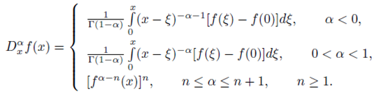 (1)
(1)
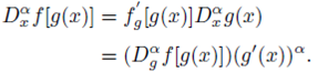
Some properties of the fractional modified Riemann-Liouville derivative are
 (2)
(2)
 (3)
(3)
 (4)
(4)
Now in order to introduce the Feng’s first integral method21, let us consider the space-time fractional differential equation with independent variables x 1, x 2,…, xm , t and dependent variable u
Using the variable transformation
where ki and c are constants to be determined later; the fractional differential equation (5) is reduced to a nonlinear ordinary differential equation
where
We assume that Eq. (7) has a solution in the form
and introduce a new independent variable Y(ξ) = Xˈ (ξ), which leads to the following system of nonlinear ordinary differential equations
Now, let us to introduce the central idea of the Feng’s first integral method. By using the division theorem for two variables in the complex domain which is based on the Hilbert-Nullstellensatz theorem 44, we can obtain one first integral to Eq. (9) which can reduce Eq. (7) to a first-order integrable ordinary differential equation. An exact solution to Eq. (5) is then obtained by solving this equation directly.
Division Theorem: Suppose that P(x, y) and Q(x, y) are polynomials in ℂ[x, y], and P(x, y) is irreducible in ℂ[x, y]. If Q(x, y) vanishes at all zero points of P(x, y), then there exists a polynomial H (x, y) in ℂ[x, y] such that
3.- Applications
The aim of this work is to obtain analytical solutions, by applying the Feng’s first integral method 20, for the space-time fractional coupled mKdV equation
where
By considering the traveling wave transformation
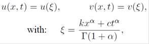 (13)
(13)
where k and c are constants, substituting (13) into Eq. (11), we can reduce the Eq. (11) into an ordinary differential equation (ODE)
For our purpose, we can consider the following ansätz
where
By adding the two Eqs. (16), the next equation is obtained
We can rewrite the above equation to obtain
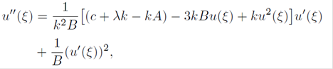 (18)
(18)
now using Eqs. (8) and (9), Eq. (18) is equivalent to the two-dimensional autonomous system u(ξ) = X(ξ) and Y(ξ) = Xˈ (ξ), where
with
Now, the solution of the Eq. (19) can be investigated by applying the Feng’s first integral method. According to the Feng’s first integral method, we suppose that X(ξ) and Y(ξ) are nontrivial solutions of Eq. (19), and Q (X, Y) is an irreducible polynomial in the complex domain ℂ, such that
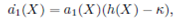
where the coefficients ai (X) (i = 0,1, … , m) are polynomials of X and am (X) ≠ 0. Due to the division theorem, there exists a polynomial g(X) + h(X)Y in the complex domain ℂ[x, y], such that
We consider the case where m = 1 in Eq. (21), by equating the coefficients of Yi (i = 2,1,0) on both sides of Eq. (22), we have
 (23)
(23)
 (24)
(24)
 (25)
(25)
since ai
(X)(i = 0,1) are polynomials of X. Balancing the degrees of g (X) and a
0 (X), from Eq. (23) it can be concluded that a
1 (X) is constant and h (X) = K = 1/B. For simplicity, we take a
1 (X) = 1. Substituting a
1 (X), and h (X) into (24) and (25), and setting all the coefficients of powers of
where a 0 (X) can be expressed as follows
and A 0 and B 0 are given by
and therefore
by taking into account the condition:
and the relation a 1 (X) = 1, from Eq. (29), it follows that
Combining this first integral Y (ξ), with the two-dimensional autonomous system of the Eq. (9), the exact solutions to the second order differential equation (18) can be obtained, and considering the relation (15), then the exact traveling wave solutions to the mKdV system (11) can be written in terms of the solution of the following first order differential equation
If we substitute this last result into any one of the Eqs. (16), (u (ξ) = X (ξ)) i.e.
the following condition required for the ansätz of the Eq. (15) is obtained
in order that the solution u (ξ) = X (ξ) satisfies the coupled mKdV equation, with
The general solution for the space-time fractional mKdV Eq. (11) is obtained by solving the first order differential equation (32), which can be written as follows
where
and X (ξ) satisfies the generalized Riccati equation (36). The generalized Riccati equation (36) has twenty seven solutions 48, which can be expressed as follows.
Family 1: When p 2 - 4qr < 0 and pq ≠ 0 (or rq ≠ 0), the solutions of Eq. (36) are
with
Family 2: When p 2 - 4qr > 0 and pq ≠ 0 (or rq ≠ 0), the solutions of Eq. (36) are
where M and N are two non-zero real constants and satisfies the condition N 2 - M 2 > 0
Family 3: When r = 0 and pq ≠ 0, the solutions of Eq. (36) are
 (42)
(42)
where
Family 4: When q ≠ 0 and r = p = 0, the solution of Eq. (36) is
where c 1 is an arbitrary constant.
For the nonlinear space-time fractional coupled mKdV Eq. (11), we have found twenty seven solutions that can be
obtained from the solutions (38), (39), (40), (41), (42) and (43) the relations (15), (37) and the condition (34).
It is worth noting that solution (38) and (39) are not of the soliton type, because they are periodical-type solutions in the variable ξ. Moreover, for the solution X 27 (ξ) it can be shown that this one does not correspond with the traveling wave solution, since the condition r = p = 0, together with the relation (37) give as a result that c = 0 and then X 27 (ξ) is not an analytical solution of the traveling wave type for the coupled mKdV equation.
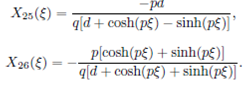
However, the solutions (40), (41) and (42) correspond to the traveling wave type soliton solutions. It can be shown that for the special case of the solution
when we take into account the relation
Substituting (37) in order to simplify the expression
and
where
Therefore the solution (45) simplifies to
 (49)
(49)
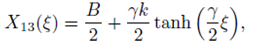
taking into account the relation u (ξ) = X (ξ) and the Eq. (15), the exact analytical solution for the space-time fractional coupled mKdV Eq. (11), is given by
with
where we have taken into account that A = -(B 2/2) + λ.
We notice that for this particular solution u (ξ) = X 13 (ξ), we have recovered the previously well known solution (50), that have been found in Ref. (43), but to the best of our knowledge the general solutions: (40), (41) and (42), that correspond to the travelling wave type soliton solution, have not been obtained previously in the literature. Since the coupled mKdV equation describes approximately the motion phenomena appearing in a two-layer fluid system 35, the new analytical solutions (40), (41) and (42) would be useful in the study of the physical behavior of these fluid systems.
Conclusions
In this paper, the Feng’s first integral method was applied successfully to obtain new exact analytical solutions of the nonlinear space-time fractional mKdV equation (11). The performance of the Feng’s first integral method is reliable and effective to obtain new solutions. This method has more advantages: it is direct and concise. Thus, the proposed method can be extended to solve many systems of nonlinear fractional partial differential equations in mathematical and physical sciences. Also, the new exact analytical solutions, Eq. (40), (41) and (42), obtained for the coupled mKdV equation can be very useful as a starting point of comparison when some approximate methods are applied to this nonlinear space-time fractional equation.

