2.1. Stationary case

The expansion of the outgoing Green’s propagator G⁺ in terms of resonant states and its connection with the scattering wave function are presented in detail in ¹⁵, and we shall recall here the main equations. The outgoing Green’s propagator G⁺ along the internal region of a one-dimensional finite range potential V(x) of arbitrary shape that extends on a finite spatial interval 0≤x≤L, and vanishes elsewhere, can be derived using the following analytical procedure. Let us consider the complex integral I in the k-plane,

along the closed contour C, where we use the fact that G+(x,x';k) is a meromorphic function of k that possesses an infinite number of complex poles k _n distributed in k-space in a well known fashion, as depicted in Fig. 1. In this Fig. 1 we also show the details of the integration contour C which is composed of a closed contour C _R of radius R about the origin in the clockwise direction which excludes all the poles {kn}, enclosed by infinitesimal small circular contours C _n, and the pole at k '=k enclosed by a circular contour C _k, where both paths are traced out in a counterclockwise direction. Using the fact that the integrand is analytic inside C, it follows from Cauchy’s theorem that I = 0, and hence Eq. (1) reads

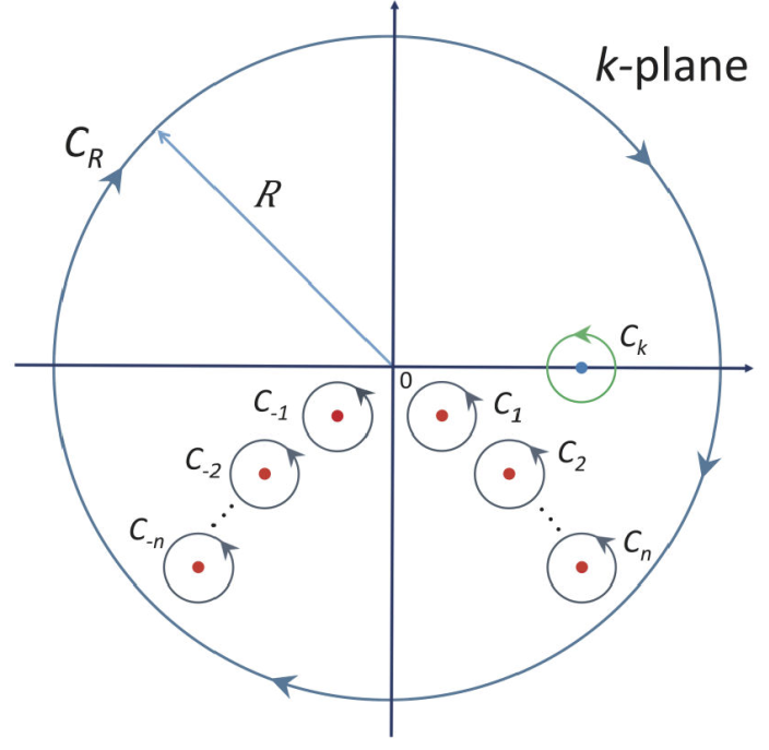
Figure 1 Closed contour C in the complex k-plane used to obtain the discrete resonance expansion of G ⁺ given by Eq. (3). The contour excludes all the complex poles of the integrand of Eq. (1), and is composed by the following contours: C_R of radius R centered about the origin in the k-plane following a clockwise direction, and C_k that encloses the pole at k = k, and all the Cn that encircle the set of complex poles {k _n} of G ⁺, both in an anti-clockwise direction. 

One may obtain the first two integral in Eq. (2) by using the residue theorem, and the fact that the residues r_n at the complex poles of G+(x,x';k') are given by rn=un(x)un(x')/kn. The last integral in Eq. (2) vanishes in the limit R→∞ due to the fact that when |k|→∞, G+(x,x';k')→0. Following this procedure, we obtain the discrete series expansion of G+(x,x';k') given by

where the index n runs on both the third (n < 0), and fourth (n < 0) quadrants. The un’s in the above equation are the one-dimensional Gamow functions, which are eigen solutions of Schrödinger’s equation,

with outgoing boundary conditions:

dun/dx|x=L=+iknun(L), dun/dx|x=0=-iknun(0).

This set of eigenfunctions {un} constitute a basis of resonance states, which obey the following normalization condition,

In order to obtain an expansion of resonance states {un} of the solution ψ(x,k) of Schrödinger’s equation along the internal region of the potential, we use the relationship between ψ(x,k), and the outgoing Green function G⁺ of the system, given by ⁹

which combined with Eq. (3), leads to the resonance expansion for ψ(x,k),

As pointed out in ¹⁶, the above expansion does not apply for the case x=x'=0. A nice feature of the resonance expansion given by Eq. (7) is that it establish a link between the spectrum of the system and the corresponding scattering problem. The information regarding the spectrum manifests itself in the set of complex poles {kn} of the system, which are distributed in the complex k-plane as shown in Fig. 2. Since in practice one considers a finite number N of resonant terms in Eq. (7), let us define the solution ψN as the truncated sum,

which will be used in our numerical calculations, testing its accuracy for different values of N. The coefficients of the sum cn(k)=ikun(0)[knk-kn]-1 provide the partial contributions of each resonance.

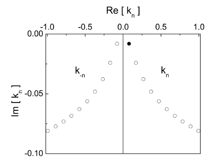
Figure 2 Distribution of the S-matrix poles of the system in the complex k-plane for a double delta potential with parameters: ¸ λ= 10:0 eV A° , and L = 30:0 A° . The poles of the third and fourth quadrant are related through -k_-n = kn* (n = 1; 2; 3; :::), which follows from time-reversal invariance. 

2.2. Dynamical case

Let us now consider the dynamical situation of incident particles on a resonant structure represented by the potential V(x). The calculation of the dynamical probability density |Ψ(x,k,t)|2 inside the system involves the solution of the time-dependent Schrödinger equation,

with H^=-(ℏ2/2m)∂2/∂x2+V(x), using the reflecting Moshinsky shutter initial condition ^15,17 at t = 0, namely

The analytical solution that involves a resonance state expansion (RSE) with explicit time dependence reads,

where ψ(x,k) is the stationary solution given by Eq. (7). The time-dependence of the solution is contained in the Moshinsky functions,

where w[iyq,t] is the complex error function , with complex argument

where q stands for ±k or k±n.

In practice, the evaluation of the dynamical solution, Eq. (11), is performed for a finite number of resonance terms N. For our numerical calculations,we define a solution ΨN(x,k;t) as

where ψN(x,k) is the stationary solution given by Eq. (8).

Equation (14) has been studied and applied mainly at the boundary point x = L since Ψ at that point relates to transport properties of the system, such as the transmission coefficient and tunneling time. In the internal region of the potential, ΨN(x,k;t) has been used to analyze the buildup process, but these analysis has been performed only in situations where the one-resonance approximation works well^12,15, which is the case of sharp and isolated resonances, i.e.|εn±1-εn|≪Γn. In a more general situation, the contribution of various resonance poles should be considered in the resonance expansion. This is the case for example of the buildup at very short times and/or at off-resonance incidence energies. Hence, an analysis of the convergence of the solution along the whole internal region is required. As we shall illustrate below, the convergence is position dependent i.e. the convergence is fast in certain points inside the system, and slow in others. In addition to the above, attention to the boundary value x = 0 is needed since the above series expansions do not apply at this point where subtractions¹⁵ are required to ensure convergence (See however Refs. ¹⁹ and ²⁰ where Cordero and García-Calderón use an auxiliary function avoiding the use of subtractions), thus a slower convergence of both solutions (11) and (7) is expected near this special point. As we shall see, the probability density exhibits this feature of the solution as a Gibbs phenomenon near x = 0.

Note that in the dynamical solution there are two kinds of convergence to be considered. One of them is its convergence to/ the stationary solution which is the asymptotic value that should be reached as t→∞. The other corresponds to the behavior as N →∞ where N is the number of resonance terms of the expansion.

3.1. Stationary case

We now analyze the convergence speed of the RSE by exploring the probability density along the whole internal region of the system. In what follows we perform a comparison of the probability density calculated with the solution given by Eq. (8) for different values of N, and the exact solution ϕ(x,k) to Schrödinger’s equation,

along the internal region. The latter is calculated by a standard approach of quantum mechanics that deals with the one-dimensional scattering of plane waves incidence from the left of the potential V (x) given by Eq. (15). The solution of Eq. (16) reads,

By computing the coefficients A (k) and B (k) by means of the well known transfer matrix technique we obtain the corresponding wavefunction for the internal region,

where we have defined κ=mλ/ℏ2.

In order to measure the degree of proximity between the curves of the probability density computed with Eqs. (8) and (18) (a procedure that involves the comparison of a large number of points) we use a computational tool that provide us with a global estimate of the degree of convergence of the probability density computed from Eq. (8) in terms of a single parameter. We introduce such a parameter p as the (percentual) global degree of convergence between |ψN(x,k)|2 and |ϕ(x,k)|2 along the whole interval 0≤x≤L, defined by

where

Insofar, as |ψN(x,k)|2 and |ϕ(x,k)|2 become alike, ξ2 will be negligible and so p will approach to 100%.

The values of the stationary probability density |ψN(x,k)|2 calculated from Eq. (8) are shown in Fig. 3 (red solid line) for an incidence energy near (and below) the first resonance, E=ε1-Γ1=0.203 eV. Here we plot |ψN(x,k)|2 vs x along the internal region of the potential varying the number N of the truncated expansion (8). Notice that this sum includes 2N resonance terms since it runs over both negative and positive n. We illustrate here the cases for N = 1, N = 4, N = 30, and N = 500. The exact probability density |ϕ(x,k)|2, calculated by a standard approach of quantum mechanics, is included for comparison (blue dashed line). As we can appreciate in the different graphs of this figure, the convergence is faster at points close to x = L, and it gradually becomes slower as we move from right to the left edge of the system. Near the point x = 0 the approximate curve exhibits a Gibbs phenomenon characterized by a series of oscillations that fade out as N is increased. The values of p for each of the cases shown in Fig. 3 are included in each graph, illustrating the improvement introduced with the increase of N. For N = 1 the approximation is far from reproducing the exact curve as we see in Fig. 3 (a).By increasing the number N of resonance terms (with the contribution of the third-quadrant poles included), a better description is accomplished as shown in Figs. 3(b), (c) and(d).

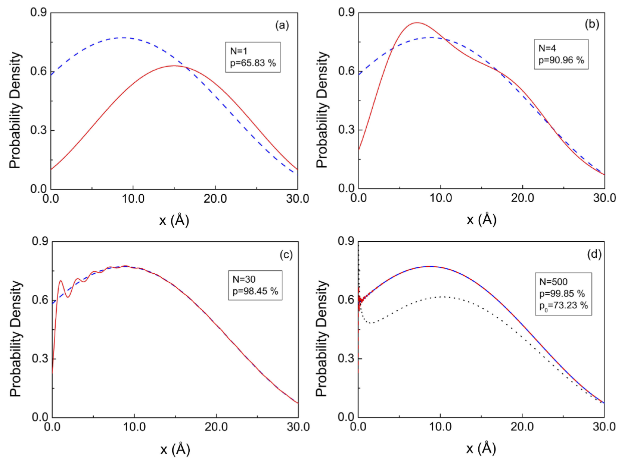
Figure 3 Comparison of the probability density of the approximate solution, Eq. (8) (red solid line), with the corresponding exact calculation, Eq. (18) (blue dashed line), at off-resonance incidence energy. The number N used in the expansion (8) and the value of p are indicated in the graphs. In (d), p is the value of p_o when the contribution of the poles k_-n is not included (black dotted line). 

The relative importance of the poles of the third and fourth quadrants in the complex k-plane, is further emphasized in Fig. 3 (d), where we have included an additional plot (black dotted line), which corresponds to the calculation of |ψN|2 where we have intentionally suppressed the contributions associated to the poles of the third quadrant, that is, only the N resonance terms with positive n were included in the sum. It is clearly evident that a poor description is obtained when the contribution of those poles is ignored. In fact, in the absence of such contributions, p reduces from 99.85% to the value p ₀ = 73.23%. The above comparison illustrates the importance of the terms with negative index in the resonance expansion [Eq. (7)].

We stress out however that there are situations in which the contributions of the third quadrant poles can be neglected. The simplest situation occurs when the incidence energy matches one of the resonances, say E=εn. In this case, we expect that the contribution of the corresponding resonance will dominate over the rest, and hence the approximation with N = 1 may be sufficient in the expansion, that is

Moreover, if the chosen resonance is sharp and isolated i.e.|εn+1-εn|≫Γn, the contribution of the pole of the third quadrant, k-n, will become negligible so that |c-n(k)|≪|cn(k)|. In such a case, the contribution of c-n(k) can be ignored, and

may provide an excellent approximation.

To illustrate this case, let as consider a symmetrical double-delta resonator with stronger barriers and the incidence energy chosen at the first resonance, E=ε1. In this example, λ=40.0 eV Å, L = 30.0 Å, and the position and width of the first resonance are ε1=0.522 eV, and Γ1=0.023 eV, respectively. This resonance is sharp enough to ignore the contribution of k _-1, in fact we have here |c1/c-1|=174.33, and the result is illustrated in Fig. 4. The approximate calculation from Eq. (22) (red solid line), using the single pole k 1 of the fourth quadrant (see full circle in Fig. 2(a)), agrees quite well with that given by the exact calculation |ϕ|2 (blue dashed line), specially in the case of sharp and isolated resonances. According to Eq. (19), the global degree of convergence is accomplished up to p = 99.73%.

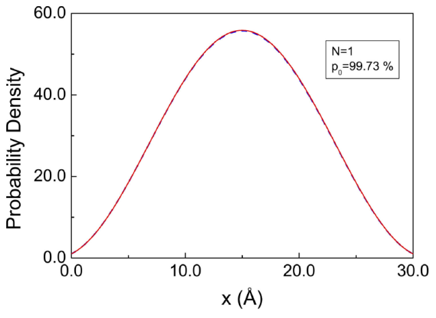
Figure 4 The one-term resonance expansion formula given by Eq. (22) (red solid line) accurately describes the exact calculation (blue dashed line) at resonance condition, E = ɛ₁ . Even though the contribution of the pole k _-1 is not included, the proximity p0 is almost 100%. 

This shows that the additional contribution from the poles k _-n of the third quadrant is not essential in this case. In the two examples discussed above, where we analyze the behavior of the resonance sum (8) as a function of N, the convergence proved to be more efficient in the system with a higher value of λL i.e. a smaller N is needed in order to accomplish a given value of p. It turns out that systems characterized by the same product λL exhibit an identical behavior, provided that the incidence energy is properly chosen. This is relevant because it can predict the behavior of families of systems with different λ and L but with the same product λL.

In order to illustrate the gradual increase of p with N, a p vs N plot is shown in Fig. 5 for the same double-delta system (which from now on we call system A), and same incidence energy (solid line). If the difference between the incidence energy and the nearest resonance is increased, more resonances are needed in the expansion to keep the proximity level. The p vs N plot for E=ε1-2Γ1=0.0580eV (dashed line) is also shown in Fig. 5. In system A, the product of the potential parameters was λL = 300.0 eV Å2. Some interesting regularities appear when we consider different systems with the same product λL. To illustrate this point, let us consider two additional systems: λ= 5.0 eV Å, and L = 60.0 Å (system B), with resonance parameters ε1=0.08732 eV, and Γ1=0.0364 eV; and λ = 3.0 eV Å, and L = 100.0 Å (system C), with resonance parameters ε1=0.0314 eV, and Γ1=0.01310 eV. The corresponding p vs N plots for the same deviations from resonance (in units of Γ1) considered in system A i.e.E=ε1-ηΓ1 (η = 1,2) are shown in Fig. 5. As we can see, all the graphs corresponding to the same value of η coincide. We have used three different symbols on the curves (a hollow dot for system A, a cross for system B, and and a vertical line for system C) and their positions on each of the curves completely overlap.

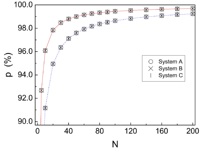
Figure 5 Behavior of p for different systems sharing the same product λL for incidence energies below the first resonance. The deviations from resonance are: Γ1 (red solid line), and 2Γ1 (blue dashed line). Notice how for a given deviation (in units of Γ1) the three systems share the same curve. 

This numerical invariance is interesting by itself, and useful for the present study since it will enable us to characterize the convergence properties of the resonance expansion for all the systems with the same λL. As we show analytically in the Appendix, the above is regularities are explained in terms of a scaling property of the Schrödinger equation (valid for these potentials) that leaves invariant ξ2 and hence the value of p.

3.2. Dynamical case

We are interested here in the analysis of the buildup process of the electronic probability density inside the system using the time-dependent solution given by the resonance expansion (14), which can describe the evolution of |ΨN(x,k;t)|2 from the transient to the stationary regime. Notice that the stationary solution ψN(x,k) is included in the dynamical expression (14), and hence the analysis of convergence performed in Sec. 3.1 is also relevant for the dynamical case i.e. its convergence guarantees the correct behavior of the first two terms in Eq. (14). However, the behavior of the sum in Eq. (14) includes both the spatial and the time dependence, and should be analyzed separately, specially at short times. Previous studies of the buildup process based on the shutter approach have been performed at resonance ^12,15, and near-resonance(12). Those studies have in common the fact that the systems fulfill the condition of sharp and isolated resonances (i.e.Γn≪|εn-εn±1| ) and not too short times, conditions that guarantees that the one-term approximation i.e. N = 1 in the expansion for ψN(x,k;t), works well. We are extending here the analysis to situations where the above conditions not necessarily are satisfied, and as a consequence the one-resonance approximation no longer applies²².

As an example, let us consider the problem of a particle of energy E incident from the left (x < 0) on a symmetrical double delta potential [Eq. (15)], with the same system parameters as in Fig. 2. In order to study the probability density in the whole time-domain, we introduce an alternative solution based on a continuum wave expansion (CWE). The latter is based on a standard approach in quantum mechanics that has been used to explore numerically²², and analytically²² the dynamical aspects of sharp wavepackets in momentum space (cutoff plane waves) in potential barriers. In the present study we have adapted the method used by Brouard and Muga²² to analyze the dynamics in the well region of the double delta potential. We begin with the following expansion²² ,

that deals with an integration of the stationary wavefunction ϕ(x,k) along the internal region, in our example given by Eq. (18), with an expansion coefficient C(k,k′) defined as,

By substituting in Eq. (24) the initial condition Ψ(x',k,0) given by Eq. (10), we obtain the result,

where ϵ is an infinitesimal positive number used to guarantee the convergence of the integrals in Eq. (24). We calculate the expression for ΨCWE(x,k,t) by using Eq. (25) into Eq. (23), and using following the identity,

where P stands for the Cauchy Principal Value. After a few algebraic manipulations, we obtain the CWE time-dependent wave function along the internal region,

Both the RSE and the CWE dynamical solutions can describe the buildup process from the transient to the stationary regime through the evaluation of the electronic probability density |Ψ(x,k;t)|2 inside the system, using respectively the time-dependent solutions given by Eqs. (14) and (27). In the evaluation of the former, the analysis of the convergence of both the stationary solution given by Eq. (8), and the sum in Eq. (14) as N→∞ is relevant here in order to guarantee the correct description of the buildup process from the transient to the stationary regime. In the evaluation of the latter, care must be taken in choosing the appropriate integration interval in order to account for all the relevant contributions in k-space to the time-dependent wave function.

The values of the time-dependent probability density |Ψ(x,k;t)|2 calculated using the RSE approach through the evaluation of Eq. (14) along the internal region of a double delta resonator are shown in Fig. 6 for an incidence energy near (and below) the first resonance, E=ε1-Γ1 = 0.203 eV, and different values of N. Here we plot |Ψ(x,k;t)|2 vs x along the internal region of the potential for different fixed times and varying the number N of resonance terms in the truncated expansion given by Eq. (14). Notice that this sum includes 2N resonance terms since it runs over both negative and positive n. We illustrate here the cases for N = 1, N = 30, and N = 500. Snapshots of |Ψ(x,k;t)|2 taken along the transient regime are shown in Fig. 6(a), (b), and (c) at the times t = 0.1τ, t = 0.6τ, and t = 1.7τ, respectively, where τ is the lifetime of the lowest resonance, τ=ℏ/Γ1=4.5 fs.

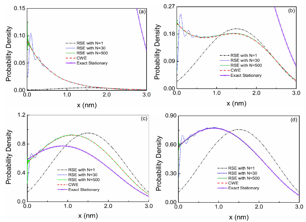
Figure 6 Comparison of the time-dependent probability density using the RSE of Eq. (14) for different number N of resonance terms with the calculation using the CWE of Eq. (27), at the fixed times: (a) t=0.1τ , (b) t=0.6τ , (c) t=1.7τ and (d) t=30.0τ, where τ = 4.5 fs is the lifetime of the first resonance. In fact, as illustrated in (d), the dynamical probability density perfectly coincides with the exact stationary value (violet solid line with crosses) in the limit of very long times. 

The calculation performed with the CWE approach, Eq. (27), is also included in these graphs (dashed red line) for the same chosen fixed times. As we can appreciate in each of these different graphs of Fig. 6, the resonance state expansion time-dependent probability density gradually converges around the asymmetric curve (CWE case) as N is increased. Since we are dealing with a scattering problem at off-resonance condition, it is expected that the resulting probability density inside the system becomes asymmetric. The symmetrical single resonance approximation, N = 1, is far from reproducing the probability density, specially at short times, as shown in Fig. 6 (a) where the contribution of the ground state becomes very small. This is because t = 0.1τ is only a small fraction of the corresponding lifetime and such a resonant state requires more time to be constructed inside the resonant structure, and the tunneling in this early stage is dominated by the higher resonances (N > 1) in a filtering process which privileges the passage of the faster components of the incident wave. As the number of resonance terms is increased to N =30, the RSE curves tend to reproduce the CWE calculation along the whole internal region of the potential except for the small oscillations (Gibbs phenomenon) near the left edge x = 0 of the system. For N = 500, these oscillations almost fade out and the RSE and CWE curves become numerically indistinguishable for long enough N. This is an interesting result not only because the formalisms beyond Eqs. (11) and (27) are quite different. A final snapshot is included in Fig. 6 (d) at t = 30.0τ, which is a sufficient long time that guarantees that the stationary situation is essentially reached at this time, as the transient regime typically extends over about ten lifetimes . Also in this asymptotic limit, the RSE and CWE calculations agree quite well for N = 500.

In order to compare with the stationary limit, we also included in each of the graphs of Fig. 6 the exact stationary probability density of the double delta potential calculated by the solution ϕ(x,k) of the time-independent Schrödinger’s equation (solid violet line with crosses). As we can see, at short times the stationary limit is still far from being reached, and only a small part of the stationary curve can be appreciated in the upper right corner of the graphs in Figs. 6(a) and (b). As time goes on, the time-dependent solutions evolve towards the stationary solution as we can appreciate in Figs. 6 (c) and 6 (d). In fact, both dynamical probability densities (RSE and CWE) become indistinguishable from the stationary case in Fig. 6 (d), satisfying the limit |Ψ(x,k;t→∞)|2→|ϕ(x,k)|2, a requirement that must be fulfilled by both dynamical solutions.

The Gibbs phenomenon observed in the vicinity of x = 0 in the RSE curves for finite N is due to the fact that the Green’s function that led to the derivation of the series expansion of Eq. (7) is not defined at the point x = 0. However, as illustrated in Fig. 6, just by increasing the number N of resonance terms to a few tens (with the contribution of the third-quadrant poles included), an excellent description can be accomplished for x > 0.

The analysis presented so far illustrates the equivalence of RSE and CWE approaches in the calculation of the internal probability density in the full time domain from the transient to the stationary regime in a typical resonant structure. One of the advantages of the RSE approach is the possibility to handle analytical expressions that allows us to study the physics of the dynamical processes more deeply. With the RSE we can analyze separately the contribution of the individual resonant states to the buildup time scales. On the other hand, using the CWE, for a given position and time we integrate numerically Eq. (27) along the k-space and obtain a single numerical value of ΨCWE(x,k;t) which involves the contributions of the whole spectrum, making no distinction among the contributions of the different resonant states of the system.