


 nueva página del texto (beta)
 Inglés (pdf)
 Artículo en XML
 Referencias del artículo
 Enviar artículo por email
 Citado por SciELO
  Similares en
SciELO
Similares en
SciELO 
 Permalink
Introduction
In the last two decades, unconventional reservoirs have become one of the ultimate frontiers in hydrocarbon exploration. These reservoirs have been mainly developed in the late Cretaceous of North America, and similar geological settings are gradually catching the attention in other petroliferous regions around the world. One of the most critical parameters to be considered during oil shale and gas shale exploitation is the amount of total organic carbon (TOC). TOC is defined as the weight of organic carbon in a unit weight of rock, commonly expressed in weight percentage (wt.%) in borehole logs. Applications of quantifying TOC can range from evaluating source rock petroleum production to kerogen typing (Steiner et al., 2016).
The late Cretaceous La Luna Formation has been reported as a high potential unconventional reservoir in northern South America (Liborius and Slatt, 2014; Ceron et al., 2013). In western Venezuela, this formation is the principal source rock for the prolific Lago de Maracaibo Basin (Escalona and Mann, 2006). In Colombia, several basins such as Catatumbo, Cesar-Rancherias, Middle Magdalena, Guajira, and Guajira Offshore also have La Luna Formation as the main source rock (Gonzalez et al., 2009). Like other organic-rich formations, TOC in La Luna is obtained from lab geochemical tests or it can be estimated from density, acoustic, and resistivity logging.
During unconventional reservoir evaluation, the most common techniques to calculate TOC from borehole logs are the methods proposed by Schmoker (1983) and Passey (1990). Schmoker and Hester (1983) proposed a method based on regression of density logging versus TOC measured in core; the method was applied in the Mississippian and Devonian Bakken Formation in the United States portion of the Williston Basin. Passey's method, also known as ALogR technique, employs the overlaying of a scaled porosity log (generally the sonic transit time) on a deep resistivity curve (Passey et al., 1990); the method is applied to assess TOC in both clastic and carbonate environments.
This work aims to provide an alternative procedure to compute TOC contents using wireline-acquired resistivity imaging and total gamma-ray log. To achieve this goal, a predictive model based on random forest algorithm was developed. This model recognizes patterns in binary and grayscale images, likewise in resistivity and gamma-ray data; using these patterns model computes TOC values along the logged sequence. The available data set has a total of 960 log measurements; these data were randomly divided into 768 samples (80%) for training and 192 for validation (20%). The accuracy of final results is evaluated through residual error, Pearson's correlation coefficient, and root-mean-square error.
The random forest, like any other supervised machine algorithm, has been successfully applied to reservoir characterization (Ao et al., 2018, Krasnov et al., 2017, Baraboshkin et al., 2019). Among the innovations presented in this work, is the application of fractal elements to train and feed a random forest model, focusing on how to supply information in the upstream oil and gas industry. Furthermore, once the predictive model is trained, this research presents a new option to calculate accurate TOC contents using only borehole imaging and gamma-ray data, providing additional value to regular borehole image interpretations.
Figure 1 presents the methodology workflow divided into two main stages, known as the training and regression (or prediction) stages. During training of supervised machines, the model utilizes a labeled dataset (independent variables), and it learns from seen results (dependent variable). Said otherwise, supervised learning is a way to use input variables (x) and an output variable (Y) to train an algorithm to learn the mapping function from the input to the output {Y = f(X)}. The goal is to approximate the best possible mapping function from input data (x) being able to predict the output variables (Y). It is called supervised learning because the process of learning from the training data set can be thought as a teacher supervising the learning process. The correct answers are known; the algorithm iteratively makes predictions on the training data and is corrected by the teacher. Learning stops when the algorithm achieves an acceptable level of performance (Brownlee, 2016). Finally, during the regression stage, the trained model must be able to figure out the dependent variable. In this case, TOC content equivalents to the TOC obtained through a semi-log regression of organic carbon measured in cores against density logging.

Geological Setting
Bralower and Lorente (2003) reported that La Luna Formation was originally named the La Luna limestone in 1926 after the Quebrada La Luna in the Perijá range. However, this unit was formally called formation in 1937; the formation consists of thin-bedded and laminated dense dark gray to black carbonaceous-bituminous limestone and calcareous shale. The limestone beds vary from a few centimeters to less than a meter in thickness. The unit is particularly characterized by hard black ellipsoidal and discoidal limestone concretions ranging from a few centimeters to almost a meter in diameter (Bralower and Lorente, 2003).
Common lithofacies in core and outcrops include planktonic and benthic bituminous biomicrites with mudstone, wackestone, and packstone fabric. Upwards, La Luna increases the strata phosphatic content and unleashed a silicification process into those beds (Sarmiento et al., 2015). These features arrangement are settled in normal marine conditions, clearly offshore, and in restricted marine environments. The relatively high sea-level event of the Turonian to Santonian in Colombia and Venezuela originated the deposition of large amounts of organic matter contained in the offshore deposits of La Luna Formation (Ceron et al., 2013). The Turonian to Santonian interval of the Cretaceous Colombian basin was deposited during a relatively fast sea level rise (transgressive systems track) and following high sea level or highstand system (Guerrero, 2002).
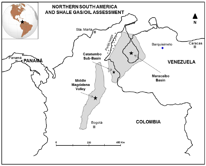
According to EIA (2015), northern South America has prospective shale gas and shale oil potential within the Cretaceous fossiliferous calcareous mudstone of La Luna Formation, particularly in the Middle Magdalena Valley, and the Maracaibo/Catatumbo basins of Venezuela and Colombia (Figure 2). The organic-rich Cretaceous shale of La Luna Formation averages 5% of TOC, and it sourced much of the conventional oil and gas produced in the Middle Magdalena basin of Colombia and western Venezuela. This formation is similar in age to the Eagle Ford and Niobrara shale plays in the United States (EIA, 2015).
Sources And Type Of Data
Resistivity imaging and average pad resistivity
The resistivity imaging can be acquired in water or oil-based muds, showing a two-dimensional pseudo image of the wellbore wall. In conductive environments, as in the case of this work, the vertical resolution of image tool is 5 mm, with 80 % of coverage in wells with 21.59 cm of diameter. Borehole imaging is applied for electrofacies classification, structural analysis, fracture characterization, thin layer identification, and direction of main horizontal stresses, among other applications. Typically, two processed images are presented from resistivity normalization, called the dynamic and static images. The dynamic image provides details, allowing recognition of sedimentary structures and classification of textural features; the static image is utilized, but not limited, to highlight resistivity changes usually related to unconformities, fluids contacts, faults, and fractures. Figure 3 shows an example of dynamic and static images in a section with limestone concretions of La Luna Formation.

Image tools are composed of assemblies of pads and electrodes, normally 20 or 24 electrodes per pad. The electrodes measure resistivity simultaneously every 5 mm along the borehole wall; the simple average of these measurements is used as a high-resolution resistivity curve (IMG_Res, Figure 3). This curve is utilized for thin layers analysis and can further be employed for petrophysical evaluations as a shallow resistivity log.
Total gamma rays (GR)
The resistivity imaging is acquired together with a GR log; this log measures the natural emission of gamma rays from radioactive elements in the formation. In Figure 3, the GR log is presented in track 3 on a linear grid and in API units (American Petroleum Institute). GRs in sedimentary sequences are mainly emitted by radioactive elements of the uranium group, thorium group, and potassium. The total GR log gives the radioactivity of the three elements combined (Rider, 2000). Among sedimentary rocks, shales have the strongest radiation, and hence the highest gamma-ray response because of the concentration of radioactive minerals. However, clean sandstone (i.e., with low shale content) might also produce a high gamma-ray response if the sandstone contains potassium feldspars, micas, glauconite, or uranium-rich water (Asquith and Krygowski, 2004). GR log is further applied to identify depth mismatching between logs acquired separately in wells.
Bulk density logs
The bulk density (pb or RHOB) is the density of the entire formation as measured by the logging tool in g/cm3 (Figure 3). This tool has a shallow depth of investigation, and it is held against the borehole during logging to maximize its response. Formation bulk density is a function of rock-matrix density, porosity, and fluid density in the pores; therefore, density log is used to quantify porosity, matrix characterization, and TOC evaluation in unconventional reservoirs. Most of the density tools are comprised of a medium-energy gamma rays source, usually cobalt 60, cesium 137, or in some newer designs, an accelerator-based source (Asquith and Krygowski, 2004).
Target or dependent variable
The target or dependent variable refers to the variable to be predicted; in the case of this study this variable is equivalent to the TOC obtained using the equation (1):
Where RHOB represents the bulk density from density logging; equation (1) was found through lab geochemical tests, using a semi-log regression between TOC in core samples against density logging values. TOC in the lab was obtained through oxidation of organic matter in core samples of La Luna Formation. Equation (1) provides a precise procedure when TOC contents need to be known from wireline logs (TOC_RHOB in Figure 3).
Fractal processing
Fractals
Benoit Mandelbrot coined the term fractal in 1975, from Latin fractus or irregular. Fractals refer to objects generated by process of repetition, characterized by having details in any observed scale, infinite length, and fractional dimension. Fractal analysis is a well-established scientific method to study natural or artificial objects that have characteristics of repetition in some form (Mandelbrot, 1983). In a statistical sense, fractals are inherent in geology domains like stratigraphy, geochemistry, and fractured rock systems; based on this property some authors have proposed the use of fractals to describe regular patterns in these domains (Schlager, 2004; Park et al., 2010; Sadeghi et al., 2014; Ayad et al. , 2019). Additionally, borehole logs represent variations in rock physical properties along the wells, and it has been documented that they can also be described through fractal parameters (Vivas, 1992; Turcotte, 1997; Arizabalo et al., 2006; Leal et al., 2016, Leal et al., 2018).
Like any other image, fractality of a resistivity image can be evaluated through its lacunarity and fractal dimension; both parameters computed after converting the image into binary (black and white). In addition to lacunarity and fractal dimension, multifractal processing of grayscale images can provide further measurements of dimension. From these analyses can be extracted variables or attributes that can later be employed as independent variables to train and feed a machine learning regression model.
Lacunarity
Lacunarity analysis is a method for describing patterns of spatial dispersion. It can be used with both binary and quantitative data in one, two, and three dimensions. Although originally developed for fractal objects, the method can be used to describe nonfractal and multifractal patterns (Plotnick et al. , 1996). Lacunarity can be considered as a measure of the relationship between not filled spaces in images. According to Quan et al., (2014), low lacunarity indicates homogeneous objects; whereas objects of high lacunarity are related to heterogeneous spaces. Allain and Cloitree (1991) proposed a method to compute the lacunarity of binary images using a gliding-box based algorithm, summarized as follows:
Take an image of side M × M (e.g., an image of 300 pixels large by 300 pixels width), and place a box of size r x r in the upper left corner (with r < M).
Count the number of black pixels in the box (box mass).
Move the box one pixel to the right and calculate the new box mass.
Repeat this process for all possible boxes over all columns and rows of the image matrix.
The number of gliding boxes of size r containing P occupied sites is taken as n(P,r), and the total number of gliding boxes of size r is taken as N(r); being M the matrix size in the equation (2):
The gliding-box masses frequency distribution can be converted into a function by dividing the gliding box count by the total number of gliding boxes. As shown the function Q(P,r) in the equation (3):
The first Z(1) and the second Z(2) moments of this distribution can be calculated employing the equations (4) and (5), respectively:
Finally, the lacunarity λ of the image for a gliding box of size r × r can be computed with the equation (6):
Fractal dimension
Fractal dimension (FD) is an effective measure for complex objects (Li et al., 2006), representing the space-filling capacity of a pattern. The FD quantifies a subjective feeling about how densely the object occupies the metric space in which it lies (Barnsley, 1993). A method to estimate FD of binary images is the box-counting algorithm; the detailed procedure can be described as follows:
The study image must be inserted in a box of side r.
This box should be divided into four boxes with side r/2, and the number of boxes covering any part of the figure N(r) must be counted.
Resulted boxes are divided again into four boxes, and the number of boxes N(r) containing any part of the figure must be recounted.
The procedure is repeated, counting the number of boxes with some part of the figure.
Afterward, plot the inverse of box size against the number of boxes with any part of the figure, with the Xj axis equal to Log(1/rj) and Yj axis equal to Log(Nj).
Finally, the slope m of the regression is the FD of the image computed with the equation (7):
Multifractal analysis
Multifractal analysis has been recognized as a powerful tool for characterizing textures in images. Several studies have shown the possibilities offered by multifractal analysis in image processing, particularly during classification of complex textures (Harrar and Khider, 2014). In this work multi-fractal analysis was applied to grayscale images, following the methodology proposed by Huang and Chen (2018). These authors propose to extract a set of features to characterize the image considering global (in the whole image) and local parameters (just in a part of the image). The global parameters provide the capacity dimension, information dimension, and correlation dimension; whereas local parameters provide the singularity exponent and a local fractal dimension, this last in a section of the image.
Independent variables generated by fractal processing
The independent variables refer to the required data to train and feed a predictive model; initially, a total of 49 independent variables are available for these tasks. Forty-seven of them are related to fractal variables, and the two remaining are the GR and IMG_Res, respectively. Fractal-related variables were computed using the dynamic image, employing images that represent borehole sections of 0.6 m high and 21.59 cm in diameter; these dimensions are represented with images of 300 pixels high by 360 pixels width (360° around borehole circumference). Calculations were made on the dynamic image every 300 pixels from bottom to top to create a log per each variable.
Fractal variables were defined according to their relations with lacunarity, fractal dimension, and multifractal analysis. For lacunarity, a group of variables was derived from the frequency distribution produced by calculating lacunarity using different r values. The rest of the lacunarity-related variables were computed using the geometric and statistical descriptions of patterns in scatter plots of lacunarity versus r; the scatter plots were for both linear and logarithmic scales. The same procedure was applied for FD variables, but in this case, the image size was varied to perform the frequency distribution and scatter plots. To evaluate the spectra of lacunarity, FD, and the geometrical relation between them, a total of15 values of r and 15 image sizes were experimentally selected. Two important reasons to highlight for this selection:
As the image size and r value increase, patterns in both scatter plots and frequency distributions are the same; just changes in slope and correlation coefficient (R) of linear patterns are observed.
The gliding-box and box-counting algorithms are a pixel-by-pixel review of a matrix; consequently, these processes with large gliding boxes or large images are computationally expensive. In other words, it will increase computation time resulting in no practical procedures.
Variables obtained from lacunarity processing
Variable 1: The image sections of 300 × 360 were transformed into sections of 300 × 300 (with size in pixels, and using morphologic transformation of image processing techniques). Then, the lacunarity was computed using the gliding-box algorithm (Allain and Cloitree, 1991), with r = 60 pixels. This procedure was applied over the dynamic image every 0.6 m along the well.
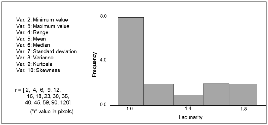
Variables 2-10: As shown the Figure 4, these variables represent the statistical description of lacunarity using several r values (r in pixels, Figure 4).
Variables 11-22: These variables are computed using the scatter plot of Lacunarity vs r. Figure 5A for a log scale (Var. 11-16), and Figure 5B for a linear scale (Var. 17-22).

Variables obtained from FD processing
Variable 23: As in the case of Variable 1, the image sections were transformed into arrays of 300 x 300, and FD was computed using the dynamic image every 0.6 m employing the box-counting algorithm.
Variables 24-32: This set of variables is related to the statistical measures of FD distribution. The analyzed section of image was resized according to the sizes in Figure 6.
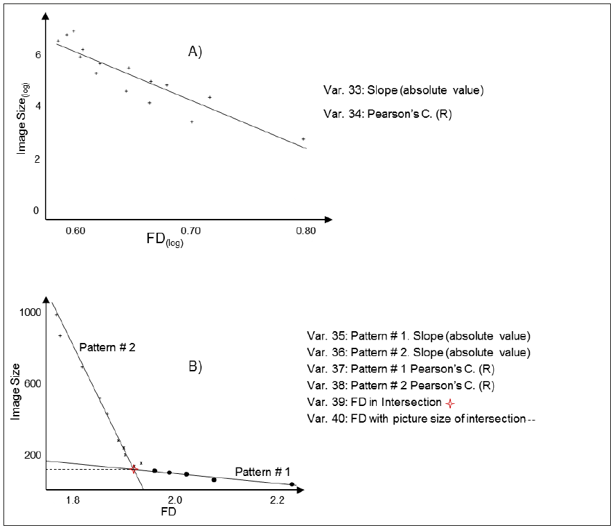
Variables 33-40: These variables are computed using the scatter plot of FD vs. Image Size. Figure 7A for a log scale (Var. 33 and 34), and Figure 7B for a linear scale (Var. 35-40).
Variables 41-42: These variables are extracted from the scatter plot of FD vs. Lacunarity, as shown the Figure 8.


Variables obtained from Multifractal processing
To compute variables between 43 and 47, image sections were transformed into arrays of 300 × 300 (like variables 1 and 23); then, they were converted from the heated scale into grayscale images. Afterward, multifractal variables were calculated every 0.6 m along the well, according to the methodology proposed by Huang and Chen (2018); these variables are described as:
Random forest
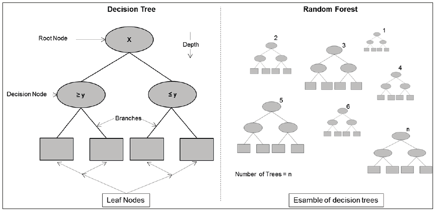
Random forest (RF) is one of the most powerful algorithms of machine learning available today. The RF is a kind of supervised learning algorithm; it uses labeled data to learn how to classify un-labeled data (Schott, 2019). This method is further categorized as an ensemble learning algorithm, due to it trains a group of decision trees and searches for the best answer among a random subset of features (Geron, 2019). A decision tree consists of just tests on features in the decision nodes, values of features on the branches, and output values on the leaf nodes (Russell and Norvig, 2010); leaf nodes are the answer or solution provided by the algorithm (Figure 9). The RF can be applied for regression and classification problems, and its processing is fast compared with other machine learning techniques; moreover, the algorithm can easily handle outliers and missing data. Common hyperparameters to be tuned in RF are the number of trees, maximum depth, and minimum samples leaf (Figure 9).
Among the RF advantages applicable to this works, and considering we are dealing with just 960 log measurements, is that RF is based on the bagging algorithm and uses ensemble learning. It creates many trees on the subset of the data and combines the output of all the trees. In this way, it reduces the overfitting problem, reduces the variance, and therefore improves the accuracy; even with a low number of samples (Kumar, 2019). Moreover, no feature scaling is required (standardization and normalization) because it uses a rule-based approach instead of distance calculation. As the main drawback, this method requires much computational power and resources during training, as it builds numerous trees to combine their outputs. However, the relatively low number of samples employed in this work helps to cope with this issue.
The accuracy of the RF was measured using Pearson's correlation coefficient and the root-mean-square error, both metrics after comparing predicted and actual values. Additionally, the distribution of residual error was employed to evaluate performance.
Pearson's correlation coefficient (R)
Pearson's correlation coefficient (R) measures the strength of linear association between two variables. The coefficient is measured on a scale with no units and can take a value from -1 to +1. If the sign of R is positive, then a positive correlation exists; otherwise, exists a negative correlation (Sedgwick, 2012). Given a pair of random variables (x,y), R is obtained using the equation (8):
Where cov represents covariance, σx and σy are the standard deviation of x and y, respectively.
Root-mean-square error
The root-mean-square error (RMSE) is widely employed to calculate the error in a set of predictions. The metric is sometimes called mean square error or MSE, dropping the root part from the calculation and the name. RMSE is calculated as the square root of the mean of the square differences between actual outcomes and predictions. Squaring each error forces the values to be positive, and the square root returns the error metric to the original units for comparison (Brownlee, 2017). The RMSE of predicted values ŷi, for samples i of dependent variables yi with n number of observations, is computed with the equation (9):
Feature selection.
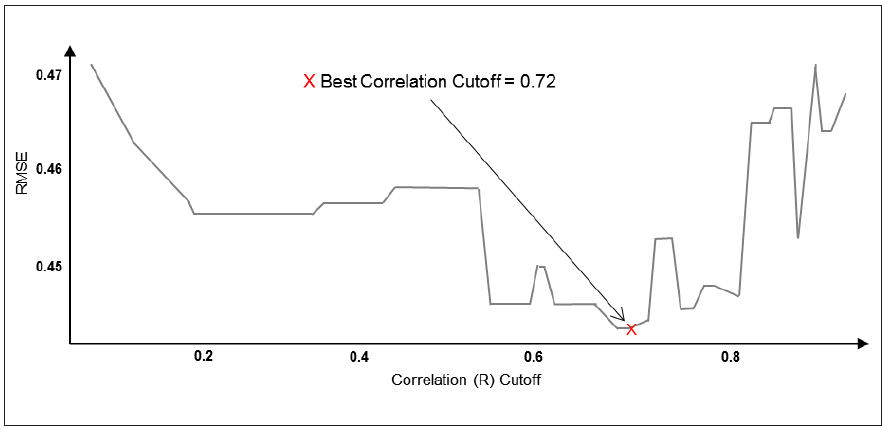
Some of the fractal variables may be providing the same kind of information to the predictive model. This duplication can increase the processing time because of high dimensionality. R is used to know the linear relationship between variables or how similar two features are; therefore, when two variables have a high correlation, one of them can be dropped from the model. In order to perform correlation analysis between variables, a cutoff must be established, and following randomly remove one of the variables with a high correlation above this cutoff.
A total of 99 RF models were executed, ranging R from 0.1 to 0.99 and removing a variable every iteration. The RMSE of each result was plotted against R, showing that the lowest RMSE corresponds to a cutoff of 0.72 (Figure 10); by applying this procedure, 32 independent variables were removed.
Feature importance.
Another quality of RF is that it makes it easier to measure the relative importance of each variable concerning the target (Geron, 2019). RF performs feature selection when it splits nodes on the most important variables. In this study, feature importance is used to decrease even more the number of independent variables and keep only the most relevant features. Extra variables can decrease performance, because they may confuse the model by giving it irrelevant data (Koehrsen, 2018).
The feature importance function was first executed to know the ranking of the remaining independent variables. Following, 16 RF models were tested to select the set of variables that produce the lowest RMSE. The less important variable was removed in each iteration, in a similar way that previous feature selection processing; after this procedure, only one variable was removed. Table 1 shows a summary and brief description of the remaining features according to their relative importance. These variables will be the input to the final RF regression model.
Table 1 Summary and description of final independent variables
| No. | Selected Variables | Description |
|---|---|---|
| 1 | GR | GR log acquired along with borehole imaging |
| 2 | Var. 43 | Capacity dimension (Multifractal Analysis) |
| 3 | Var. 11 | |Slope| - Pattern # 1 in Figure 5A |
| 4 | Var. 9 | Kurtosis of lacunarity distribution (Figure 4) |
| 5 | IMG_Res | Average resistivity curve computed with pads of image tool |
| 6 | Var. 47 | Local fractal dimension (Multifractal Analysis) |
| 7 | Var. 44 | Information dimension (Multifractal Analysis) |
| 8 | Var. 15 | R - Pattern # 2 in Figure 5A |
| 9 | Var. 1 | Lacunarity of dynamic image each 0.6 m (r = 60 × 60 pixels) |
| 10 | Var. 23 | FD of dynamic image each 0.6 m |
| 11 | Var. 38 | R - Patter # 2 in Figure 7B |
| 12 | Var. 40 | Fractal dimension using picture size of intersection (Figure 7B) |
| 13 | Var. 25 | FD maximum value (Figure 6) |
| 14 | Var. 33 | |Slope| in Figure 7A |
| 15 | Var. 13 | |Slope| - Pattern # 3 in Figure 5A |
| 16 | Var. 20 | R - Patter # 2 in Figure 5B |
Results and Discussion
After the feature importance review, the doughnut chart in Figure 11 shows the relative importance and amount of information gain provided by each variable to the predictive model. The inner ring shows the percentage of information provided for each fractal analysis; the gamma-ray and average pad resistivity are presented as a whole group in this ring. The outer ring graphically depicts the information provided for each independent variable according to their relation to lacunarity, fractal dimension, and multifractal processing; additionally, this ring shows information provided for the gamma rays and average pad resistivity separately. The exact values of information gain for each variable are presented in the table next to the doughnut chart.
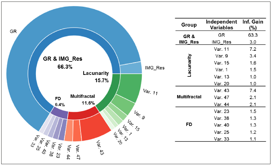
In decision trees, information gain is based on the decrease in entropy after the data set is split on a node; in other words, information gain due to a feature summed across all the levels of decision tree determines its feature importance. This can also be seen from the fact that at every node splitting is done on the feature which maximizes information gain (Singh, 2019). In accordance with Figure 10, the most important independent variable is the gamma rays log (63.3%); this is an expected result and makes geological sense because of the high uranium content in the organic matter of La Luna Formation. The following set of variables is related to lacunarity processing, which is providing 15.7% of information to the regression model.
When a section of a borehole image is binarized, the lacunarity measures relationships between high resistivity spaces in that section of the image. As was seen in the description of La Luna Formation, concretions and calcareous beds are common high resistivity features of this unit; such features appear as white spaces after the image is converted into black and white for lacunarity processing. Another fact to highlight is the amount of hydrocarbon and organic matter in these rocks; organic-rich lithologies produce light tones when borehole imaging is presented using a heated scale. Therefore, image sections in this material will be increasing the number of white pixels after binarization. These statements explain why lacunarity processing plays an important role in pattern recognition in La Luna Formation. Figure 12A shows a linear trend confirming this interpretation; in this example the micronormal resistivity log (MNRL) was compared against the variable 11 (the most important lacunarity variable).
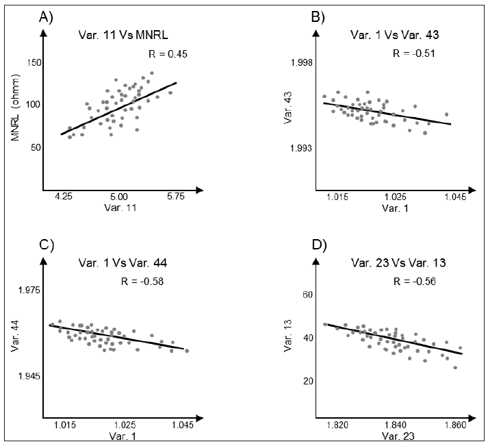
Figure 12 A) Shows a linear trend between Var. 11 (related to lacunarity) and a micronormal resistivity log (MNRL). B), C), and D) likewise show linear trends between several high-ranked independent variables related to conductivity in borehole imaging.
On the other hand, multifractal analysis is employed in this work to identify patterns in the transition from white to black or vice versa; being the capacity dimension the most important variable of this set (Var 43 with 7.4% of information gain). The capacity dimension is part of the global parameters used to describe spatial complexity, reflecting features from an overall perspective (Huang and Chen, 2018). This dimension is likewise computed using the box-counting algorithm, but in this case, the intercept is fixed to zero to avoid values greater than 2 (abnormal values). The capacity dimension is bound to be greater than the information dimension and both greater than the correlation dimension; in this work, that condition is accomplished along all logged sections. The main observations to point out about the capacity and information dimensions are the linear trends presented in Figures 12B-12C. Negative slopes in these figures suggest that multifractal parameters are complementing the information provided by lacunarity in a contrary direction, in other terms, they are related to conductivity. Multifractal parameters are describing patterns in not-resistive shelly sections or other conductive structures in the borehole image.
Finally, similar to multifractal parameters, the FD processes are related to conductive features; Figure 12D shows a negative slope supporting this interpretation. Likewise, this is an expected result because FD was computed using the box-counting algorithm, but without fixing the intercept to zero. It is important to notice that information provided by FD processes is not duplicating the information provided by multifractal variables. According to feature selection processing, these groups of variables are statistically different; the main reason is that FD was computed using binary images instead of grayscale images as in the case of multifractal processing.
Once all required independent variables are identified, the hyperparameters for the RF predictor must be established. In this study, the model hyperparameters were tuned using a grid-searching approach. Grid-searching is the process of scanning the data to configure optimal hyperparameters for a given model. Grid-searching builds a model on each hyperparameter combination provided and stores a model for each combination (Lutins, 2017). The grid-searching shows an optimal hyperparameters combination of 140 trees with a maximum depth of 35 levels and minimum samples leaf of 1. Lastly, with the optimal hyperparameters already established, the RF model was executed using the test data set, composed of 192 unseen samples. The final performance showed an R of 0.88 and RMSE of 0.44 %, as indicated by the regression in Figure 13A.
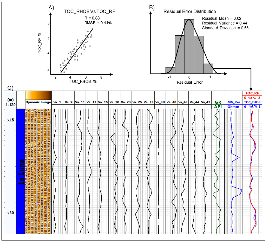
Figure 13 A) Scatter plot (TOC_RHOB Vs. TOC_RF); B) residual error distribution, and C) example of a composite log with borehole dynamic imaging, the RF input variables, and comparison between the final result (TOC_RF) and actual TOC data (TOC_RHOB).
According to the central limit theorem, the residual error of a regression model must follow a normal distribution with constant variance and zero means (Martin et al., 2017). The residual error produced by the RF model in this work presents a normal distribution as shown the Figure 13B, with a mean of 0.02 and a variance of 0.44 (equivalent to RMSE). Figure 13C shows a graphic example of input variables, dynamic image, and TOC curves (TOC_RF from the regression model and TOC_RHOB from the density log).
In order to compare the outcome of this works with other methods commonly applied to compute TOC using borehole logs, the standard deviation value is utilized. Schmoker and Hester (1983) reported an average standard deviation of 2.7 wt.% in 266 analyzed samples; these samples come from the upper and lower member of the Bakken Formation in the Williston Basin of North America. In another hand, Passey et al. (1990) reported an average standard deviation of 1.2 wt.% in 112 analyzed samples, coming from six wells drilled in organic-rich lithologies in clastic and carbonate environments. Figure 13B presents a lower standard deviation compared with these works (0.66 wt.%), which can be interpreted as less dispersion in the final results. This finding along with the R and RMSE previously explained confirms that this result can be employed during TOC evaluation in La Luna Formation.
Conclusions
The methodology presented in this research provides an alternative to evaluating TOC content soon after the image log is acquired. Only a dynamic normalized image, the total gamma rays, average pad resistivity, and fractal variables derived from image pixels are required for the entire processing. This RF predictor presents RMSE less than 0.5%, about the TOC obtained through the equation (1); furthermore, this procedure shows a lower standard deviation compared with the most common methods applied when TOC content needs to be assessed from borehole logs.
The performance of this method is sensitive to image quality, and therefore quality control of imaging data is recommended. Wireline imaging tools are based on several kinds of pad/flap configurations, and their proper operability will depend on the pad's contact with the formation. In this sense, irregular borehole sections (e.g., with breakout or washout) will produce poor-quality images, which increases the RMSE of estimated values.
The presented model was developed for vertical wells, using resistivity imaging acquired with wireline in water-based mud. Thus, the model must be recalibrated in case it is used in oil-based mud environments, in deviated or horizontal wells, and when logging while drilling imaging is employed. Further calibrations are required when it is utilized in other unconventional plays different from La Luna Formation; once recalibrated, its results can be used for choosing candidates in hydraulic fracturing programs.
The methodology presented in this work demonstrates that accurate numerical values can be decoded from the intensity of pixels in a set of images. Further research in this field is recommended; this procedure might be applied to estimate any other petrophysics attribute, such as porosity, permeability, resistivity, and saturations, among other variables.

