


 text new page (beta)
 English (pdf)
 Article in xml format
 Article references
 Send this article by e-mail
 Cited by SciELO
  Similars in
SciELO
Similars in
SciELO 
 Permalink
Introduction
Shear wave velocity plays an important role in designing the earthquake-resistant structure for any major engineering construction. Average shear wave velocity at thirty-meter depth (VS30) that is calculated from the shear wave velocity profile is a major requirement for designing an earthquake-resistant structure. The dynamical properties of the local subsoil are a major requirement for the design of earthquake-resistant structures (Amico et al., 2008, Kramer, 1996). This information can be obtained through invasive and time-consuming techniques like drilling, down/cross-hole measurements, etc. These, however, supply local information, and a satisfactory survey may result very expensive, preventing their widespread application (Amico et al. 2008). Additional problems arise when urban areas or inaccessible terrain are of concern, where invasion is generally made difficult by buildings or highly inaccessible terrain. This need has resulted in the development of a fast and cost-effective quantitative method aiming at the seismic characterization of subsoil over wide areas by the use of non-invasive procedures (Amico et al., 2008). Active and passive seismic techniques represent a good opportunity in this direction. Because of their importance, these methodologies have been recently the object of active research in the seismological (e.g., the Site Effects Assessment using Ambient Excitations [SESAME] European project, http://sesamefp5.obs.ujfgrenoble.fr/index.htm, last accessed March 2008) and engineering (North Atlantic Treaty Organization [NATO] SfP Project 980857, http://nato.gfz.hr, last accessed March 2008) field.
The geotechnical and seismic characterization of shallow soil can be made by the analysis of the surface and interface waves. Through the analysis of the dispersion properties of Rayleigh, Love, Scholte, or Stonely waves, it is possible to retrieve shear-wave velocity profiles in any region. This can be done by using waves generated from active sources as in Spectral Analysis of Surface Waves (SASW, Nazarian and Stokoe, 1984), Multichannel Analysis of Surface Waves (MASW, McMechan, and Yedlin, 1981; Park et al., 1999), Multiple Signal Classification (MUSIC, Schmidt, 1986), Multi-Offset Phase Analysis Of Surface Wave Data (MOPA, Strobbia, and Foti, 2006), and similar geotechnical approaches (Mulargia et al., 2015) or waves from passive ambient noise, as in the 2D arrays of Spatial Autocorrelation method (SPAC, Aki, 1957) and Extended Spatial Autocorrelation Method (ESAC, Ohori et al., 2002) or in the 1D of Refraction MicrotemorTM (ReMiTM, Louie, 2007) and Statistical Self Alignment Property (SSASP, Mulargia and Castellaro, 2013). Although the dispersion curve gives better results there is always chance of error in using the dispersion curve as the sole criteria due to constraints in high-frequency sources and limitations in inversion strategy.
The HVSR method, proposed by Nogoshi and Igarashi (1970) and promoted by Nakamura (1989), and standardized within the SESAME Project (2004), is the most common technique to experimentally assess the subsoil resonance (i.e., amplification) frequencies. In recent years, the joint fit of HVSR and dispersion curves have been proposed by, Parolai et al., 2005; Picozzi et al., 2005; Castellaro and Mulargia, 2010, 2014; Roser and Gosar, 2010; Zor et al., 2010; Foti et al., 2011. The joint fit of the HVSR and dispersion curve are considered better constrained than models based on the match of the curve from a single technique (Castellaro, 2016). A reliable estimate of the shear wave profile obtained at any site can give an accurate estimate of earthquake-resistant design parameters. Shear wave velocity is a diagnostic engineering tool because of its dependence on pore saturation and is considered an important tool in designing buildings for site-specific conditions such as soil liquefaction, ground-spectral earthquake response, etc. (Gorstein and Ezersky, 2015).
The state of Uttarakhand in India falls in the highest vulnerable zone IV of the seismic zonation map of India. Besides being a major source of tectonic earthquakes, it is a locale of many turbulent rivers and tourist destinations. Due to its techno-economic importance to the region, the whole area is a locale of many ongoing major civil projects including major railway projects proposed from Rishikesh to Karnaprayag. The shear wave velocity profile in this has been estimated using non-invasive active and passive seismic methods which include methods dependent on HVSR and dispersion curves. Geological bore logs in this area at the site of seismic investigation have helped in constraining the model obtained from the joint fit of dispersion and HVSR curves. The main objective of this paper is to present a detailed analysis of the shear wave profile obtained at various sites in this project and present the relation of shear wave velocity with rock type obtained at different depths for estimation of the seismic section from rock type exposed in this part of Himalayan Terrain and thus can be used for mitigating region’s seismic risk.
Geology of Region
In the Garhwal Himalaya, litho-tectonic units range in age from Precambrian metamorphic to Neogene sediments (Khattri et.al,1989). The Alaknanda River traverses through these litho-tectonic units in the Garhwal Himalaya. The Garhwal Himalaya, drained by the Yamuna, the Bhagirathi, and the Alaknanda rivers constitutes the middle part of Burrard's and Gansser's Kumaun Himalaya extending from the Sutlej to the Kali river (Khattri et.al, 1989). Garhwal Himalaya, comprising the central portion of the Himalaya, is a seismically active region of the Indian subcontinent. It is characterized by the presence of two active fault systems, namely, the Main Boundary Thrust (MBT) and Main Central Thrust (MCT), along with several minor tectonic lineaments.
The main rock types in this area are quartzite, phyllite, meta-volcanic, meta basics, and dolomites with strike directions varying from NE-SW to NW-SE. The geological map of the region together with the study area is shown in Figure 2. Quartzites are the major rock type in the area, followed by phyllites and other rocks. Quartzites and dolomites are generally hard and massive in this region except in places where thrust, fault, or shear zones are present. Phyllites and meta basics are of lower strength and have been reduced to powdery material near shear zones. In general, phyllites occupy the southern part of the area close to the North Almora Thrust (NAT) and are commonly crushed, sheared, and crumpled into numerous folds, whereas the quartzites are hard and compact with joints and fractures (Sarkar et al., 1995). A detailed geological map of the study area together with the location of boreholes at which bore log data is available is shown in Figure 2.

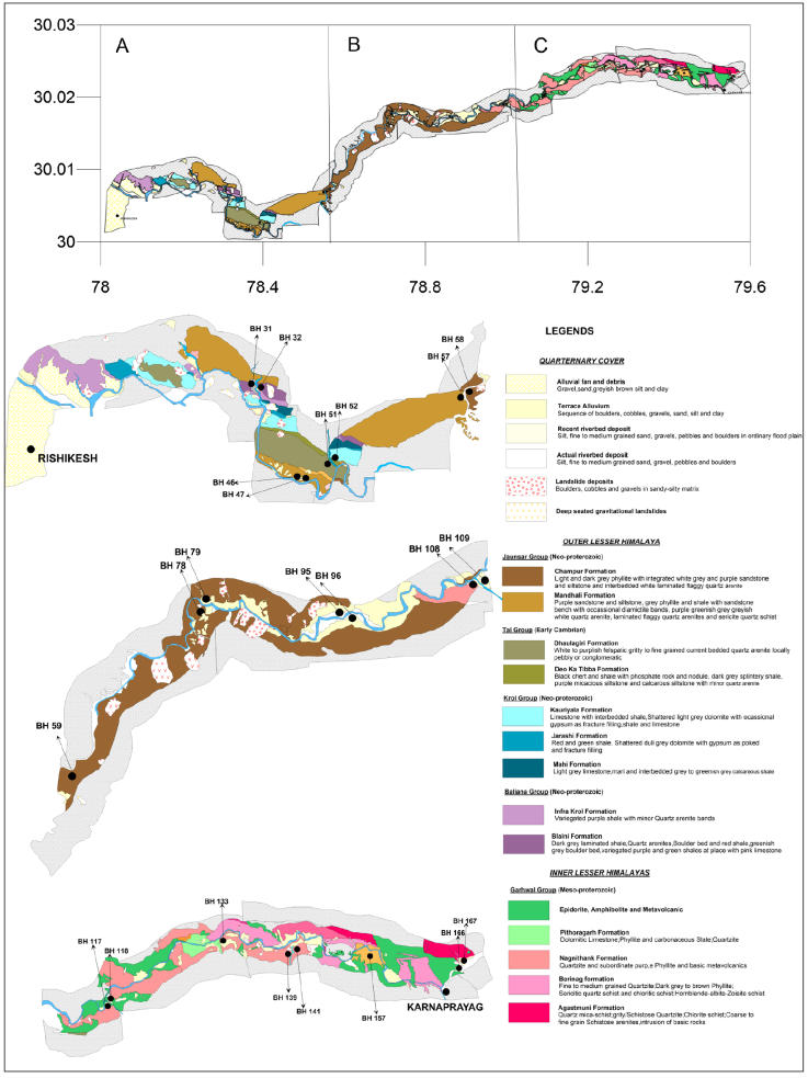
Figure 2 Location of boreholes on the geological map in the study area is shown by a rectangle in Figure 1.
Estimation of Shear Wave Velocity
One of the most common methods of obtaining shear wave velocity is based on ambient micro-tremor data. The micro-tremor data is recorded at each site by a three-component sensor having a natural frequency, which is designed to record the ambient noise. Out of three components, the vertical component is free from any kind of site effect and contains information about the anthropic activity (>2Hz) (Castro et. al., 1997). The ratio of Fourier spectra of horizontal with vertical motion carries site information. This method is popularly known as the HVSR technique. Nakamura (1989) proposes the Horizontal to Vertical Spectral Ratio (HVSR) technique, which is a non-invasive technique in the geophysical field, which gives us the shear wave velocity structure. In addition, due to its low cost, this technique is extensively used in the study of ground motion amplification at a site and gives the resonant frequency of the subsoil layer. HVSR technique is applied over a wide area of ground motion amplitude in the range from micro-tremor to strong motion (both ambient noise and weak motion recordings). Nakamura (1989) assumed that the ambient noise is generally composed of body waves but there are other cases where the ambient noise is treated as fully composed of SH waves (Mucciarelli and Gallipoli, 2004) and surface waves (Rayleigh and Love wave) (Fäh et al. 2001, Lachet and Bard, 1994). However, the surface wave content in the ambient seismic noise has been adopted in the present study and the analysis of the HVSR curve has been done accordingly.
The ratio of amplitude spectra of horizontal and vertical components constitutes the HVSR curve. This ratio has effective normalization power which removes the effect of the source and intensifies the subsoil response (i.e. path) (Nogoshi and Igarashi, 1970; Nakamura, 1989). The HVSR curve results in a peak in which the peak frequency indicates the resonant frequency (f 0) and peak amplitude indicates the amplification factor. The relation between resonant frequency (f 0), shear wave velocity (V S ) and thickness of layer (H) is given as:
Where,
f 0 is the resonant frequency of the subsoil layer (Hz),
V S is the shear wave velocity of the subsoil layer (m/s),
H is the thickness of the layer (m).
When the HVSR curve has only one single peak, it gives the correct amplification value. In the case of several peaks, the peak at the lowest frequency is the fundamental mode and the other peaks are due to the other lithologies, which cause amplification (Tsuboi et al., 2001).
In this paper, the TROMINO instrument is used as the sensor for acquiring the data. The data is generally recorded for a time length and is acquired at both ends of the linear array. In this work, GRILLA software designed by MOHO Science & Technology Company, Italy has been used for processing micro-tremor data. Fourier Spectra of all the three components of recorded ground motion are calculated and the average of two horizontal components is estimated as shown in Figure 3(b). The ratio of average horizontal spectra with vertical spectra using Eq. (1) gives the HVSR spectral ratio as shown in Figure 3(c). The portion of ambient noise data utilized for the HVSR study has been from the frequency-time plot of HVSR data of complete record shown in Figure 3.
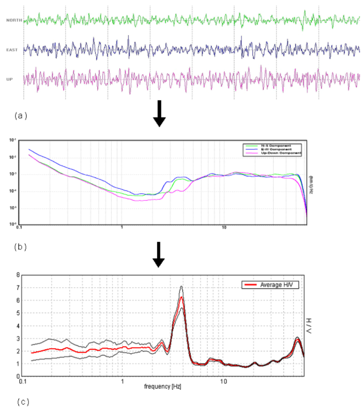
Figure 3 (a) Three-component record of ambient noise (b) The Fourier spectra of the recorded ambient noise (c) The horizontal to vertical spectral ratio (HV) curve.
Direct inversion of HVSR curves gives the shear wave velocity model but it requires knowledge of soil parameters (e.g. Poisson’s ratio and damping constant in each layer) which is not an easy task to determine. The inversion process also requires the initial model for the construction of the shear wave velocity model. The non-uniqueness in the solution obtained from HVSR inversion can be constrained by jointly fitting the HVSR curve with the dispersion curve obtained from the method commonly known as MASW. MASW is a geophysical method that is used for the estimation of shear wave velocity profile. This technique uses the property of dispersion of surface waves in elastic media. The basis of all of these techniques is the slant stack (or the correlation) of the signal recorded from different receivers, which permits the determination of the propagation velocity of waves of different frequencies travelling between them. In this method, the seismic signal is recorded at different positions (a minimum of two) over time (Figure 4a). The recorded signals are processed by slant stack and fast Fourier transform (FFT) procedures to produce the so-called phase/ group velocity spectra or dispersion curve (Figure 4b). The slant-stack adds traces by shifting it in time in proportion to its offset. The FFT of the traces produces the phase velocity spectra. Phase velocity spectra indicate the most probable velocity of the surface waves at each frequency. From this curve, a forward or inverse modeling procedure is applied to reconstruct a shear wave velocity model for the surveyed area (Figure 4c). The shear wave velocity is linked to the Rayleigh and Love wave velocity (normally 10%-15% larger) through the Poisson’s ratio, as formulated in the elastic theory of waves (Castellaro, 2016). These dispersive waves propagate with different velocities. Long-wavelength propagates with higher velocities due to its propagation from the deeper part of the earth and vice versa. Surface waves have high signal-to-noise (S/N) ratio, therefore it is used to characterize near-surface structures.

Figure 4 (a) Recorded traces at different receivers in the increasing order of distance (b) Selection of window (c) Rayleigh wave phase velocity spectra obtained from the selected window (d) Theoretical dispersion curve selected for velocity model (e) Three-component record of ambient noise. (f) HV curve from the amplitude spectra of the ambient noise (g) Velocity model was selected for the theoretical HV curve and dispersion curve.
In the present work, seismic signals have been recorded at different receiver positions using a sledge-hammer of 8 kg weight. The time series recorded at different positions of receivers in increasing order is shown in Figure 4a. The dispersion of the surface wave is visible in the enlargement of the wave packet shown in a quadrilateral window in Figure 4b. The slant stack and Fast Fourier transform have been applied to obtain the dispersion curve of the Rayleigh wave shown in Figure 4c. Ubiquitous ambient noise data recorded from a passive source (Figure 4d) at the same site has been used for estimation of the HVSR curve (Figure 4e) using the Fast Fourier Transform of the recorded signal. In this work, the seismic traces are analyzed using GRILLA software, which generates the dispersion curve. An initial velocity model is heuristically selected to obtain a theoretical HVSR and dispersion curve, which matches with field data shown in Figure 4e and c, respectively. The GRILLA software models the HVSR and dispersion curve using the forward approach by visually fitting both curves. MASW gives the best estimation of shear wave velocity at shallow depths but it does not give information about deeper parts. Therefore, it is generally modeled together with the HVSR curve to get a better-constrained shear wave velocity structure. Experimental evidence indicates that the active techniques usually provide better results in the high-frequency range, that is, shallow depth. The passive techniques that rely on ubiquitous ambient noise have the theoretical potential to perform better in the mid-to-low frequency range that is pertinent to mid-to-large depths (Castellaro, 2016). Therefore, both active and passive technique used in this paper provides reliable results in both shallow and intermediate depths.
Data Acquisition and Analysis
The study area is located in the state of Uttarakhand, India, and is shown in Figure 1. Borelog data at those sites at which seismic data using MASW and HVSR survey has been collected is shown in Figure 2. Logs have been obtained using the method of drilling. Twenty-four sites that contain geological logs have been used in this work. The data has been acquired by the TROMINO (MOHO s.r.l.) instrument to study the velocity variation at a site using joint inversion of HVSR and dispersion curve. It is a high-resolution all-in-one system for passive and active seismic surveys and vibration monitoring. It is equipped with 3 channel recording with a frequency range from 0.1-1024 Hz. The same instrument has been used to record the ambient noise and active MASW data. In the present study, the ambient noise data has been recorded for a time window of 8-10 minutes at a sampling rate of 128 Hz. This data has been further analyzed by dividing the time window into 20s duration by taking data free from anthropogenic noise. After that data has been further corrected for baseline correction using a triangular window. The resonance frequency is obtained by averaging the HVSR curves from all windows using the Nakamura technique (Nakamura, 1989). Similarly, MASW data has been recorded at each site at a sampling rate of 512 Hz. In this survey, the TROMINO is placed at a fixed position and the source has been moved to different offsets of equal intervals (1-3 m). The Sledgehammer of 8 kg and an iron plate have been used as a source and at each shot, the trigger is used. Geological samples obtained from bore log data include sandstone, clayey sand, boulders of quartzite, and phyllite with various combinations.
Shear wave velocity profiles have been obtained from the data collected by ambient micro-tremor recording instrument, using an active and passive seismic method at twenty-four different sites. In the present work, joint inversion of the HV curve and dispersion curve has been made by using GRILLA software and is shown in Figure 5. Different modes of dispersion curves have been observed in the data taken in the present study. However, the dispersion curve corresponds to the fundamental mode that has been selected for the analysis. The curve presenting the low-velocity values at each frequency is selected as a fundamental mode. In Rayleigh wave arrays, the depth of investigation is proportional to the maximum exploring wavelength divided by a number comprised between 2 and 3 (where the exact value depends on the Poisson’s ratio (Jones, 1958, 1962; Abbiss, 1981). The maximum exploring wavelength is derived from the phase velocity spectra by dividing the (usually maximum) correlation velocity by the corresponding frequency. As an example, in Figure 12a, the maximum velocity that can be observed from the dispersion curve is 250m/s at 5 Hz, which equates to a wavelength λ of 250/5=50 m and a depth of exploration of approximately 50/2.5=20 m. The velocity model up to the depth of 20 m is well explained by the joint fit of HVSR and dispersion curve and below this depth, only the HVSR curve is accountable for obtained velocity model.

Figure 5 (a) Shear wave velocity profile at Kudiyala (b) Comparison of HV curve from field data and that from velocity model shown in (a) (c) Comparison of dispersion curve from MASW survey and that from velocity model shown in (a)
The shear wave velocity section obtained from joint inversion is correlated with lithologs obtained from borehole data at twenty-four stations. The correlation of lithologs with obtained shear wave seismic profile at twenty-four stations is shown in Figures 6-9.
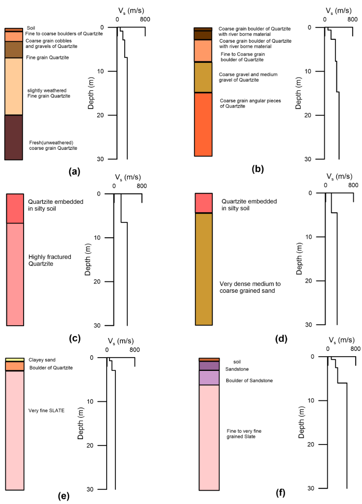
Figure 6 Shear wave profile and geological section from well log at (a) BH 31 (b) BH 32 (c) BH 46 (d) BH 47 (e) BH 51 (f) BH 52 sites, respectively
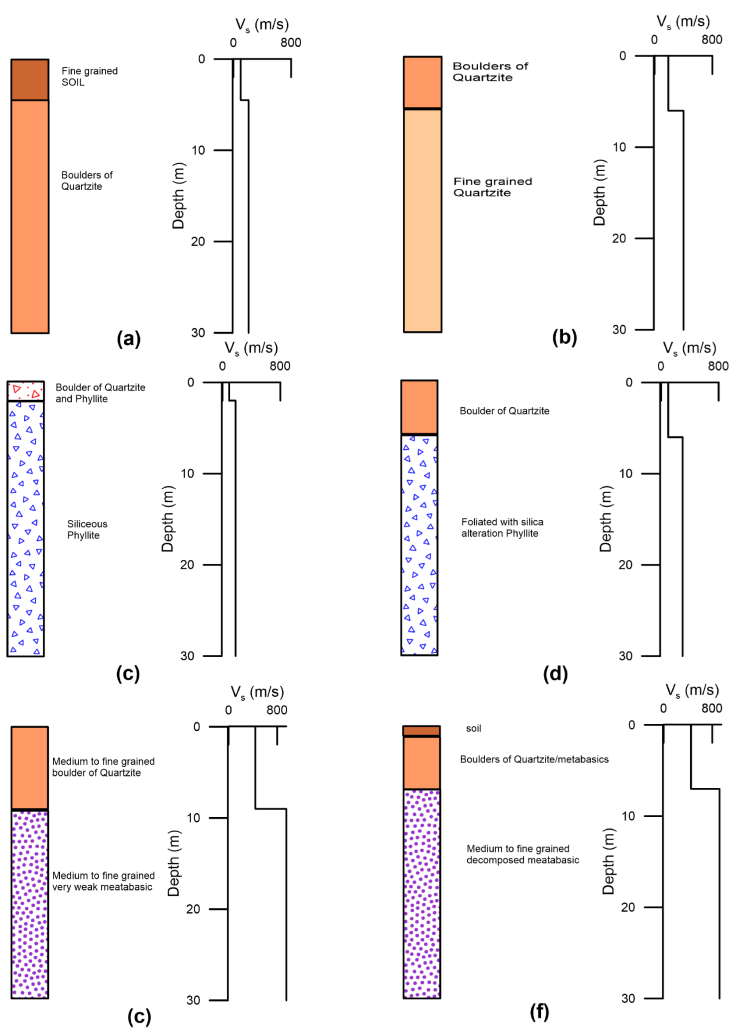
Figure 7 Shear wave profile and geological section from well log at (a) BH 57 (b) BH 58 (c) BH 59/1 (d) BH 59/2 (e) BH 78 (f) BH 79 sites, respectively

Figure 8 Shear wave profile and geological section from well log at (a) BH 108 (b) BH 109 (c) BH 114 (d) BH 115 (e) BH 117 (f) BH 118 sites, respectively

Figure 9 Shear wave profile and geological section from well log at (a) BH 139 (b) BH 141 (c) BH 157 (d) BH 158 (e) BH 166 (f) BH 167 sites, respectively
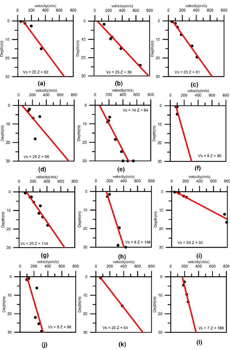
Figure 10 Shear wave velocity with respect to depth of different stratigraphic units. (a)Sand (b) Medium to the fine-grained boulder of quartzite (c) Medium to the coarse-grained boulder of quartzite (d) Fine to coarse-grained boulder of quartzite (e) Fine grained weak decomposed Phyllite (f) Fine grained soil (g) Coarse grained boulder of quartzite (h) Boulder strata medium to coarse grained (i) Medium grained sandstone (j) Fine to medium grained boulders (k) Clayey Sand (l) Boulder strata coarse grained, respectively
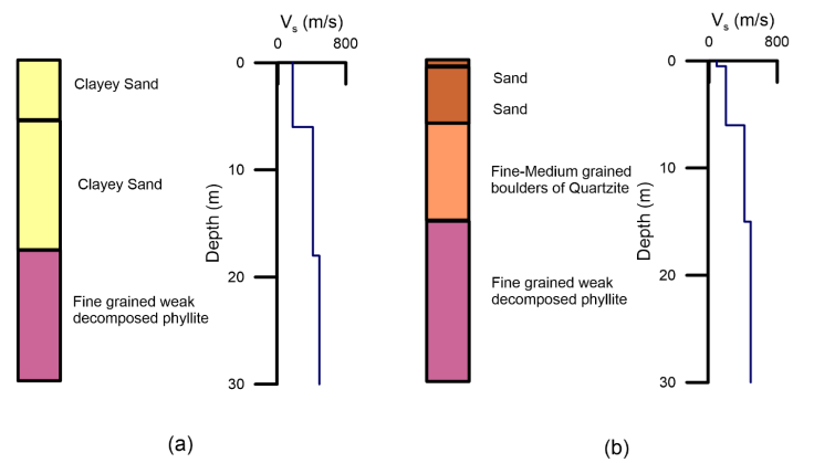
Figure 11 Shear wave velocity profile calculated from developed relation at (a) BH 95 (b) BH 96 site, respectively
Regression Model
Rock samples obtained from various logs at different stations clearly shows that similar rock type can be found at different depths, which can result in different shear wave velocities of similar rock type due to difference in their formation condition. As the modulus of rigidity increases with depth, the shear wave velocity also increases with depth. Therefore, a regression model, which defines an increase in shear wave velocity with depth, has been assigned to represent the shear wave velocity (Vs) of a particular rock type concerning its depth of formation (z) as follows:
In the above expression, the depth (z) represents the shallowest depth of rock type in meters. After obtaining a reliable subsurface shear wave velocity model from MASW and HVSR survey a database of shear wave velocity of different rock types at different depths has been obtained, for the region of Garhwal Himalayas. Linear regression relation for the model given in Equation (1) has been obtained by the least-square fit method. The best-fit line obtained for the different stratigraphic unit that follows the least square fit is shown in Figure 10. To check the efficacy of the developed relation following root mean square error (RMSE) between calculated and observed shear wave velocity has been calculated:
Here, Vs, i = Observed shear wave velocity from seismic survey
Vrel, i = Shear wave velocity obtained from developed regression relation.
The regression model and obtained RMSE for each data set are given in Table 1. It is seen that RMSE obtained for different data sets varies from five to twenty-eight m/s, which is relatively small enough keeping in view of observed velocity of rock type.
Table 1 Relation between shear wave velocity and depth for different lithological units in the Garhwal Himalayas within the depth of thirty meters
| S. No. | LITHOLOGY | RELATIONS | RMSE (m/s) |
|---|---|---|---|
| 1 | Sand | VS=20Z+82 | 21 |
| 2 | Medium to fine grained boulder of quartzite | VS=25Z+36 | 17 |
| 3 | Medium to coarse grained boulder of quartzite | VS=20Z+61 | 9 |
| 4 | Fine to coarse grained boulder of quartzite | VS=25Z+56 | 28 |
| 5 | Fine grained weak decomposed phyllite | VS=14Z+64 | 17 |
| 6 | Fine grained soil | VS=8Z+80 | 7 |
| 7 | Coarse grained boulder of quartzite | VS=20Z+114 | 14 |
| 8 | Boulder strata medium to coarse grained | VS=8Z+148 | 18 |
| 9 | Medium grained sandstone | VS=50Z+50 | 22 |
| 10 | Fine to medium grained boulders | VS=8Z+98 | 16 |
| 11 | Clayey sand | VS=20Z+54 | 6 |
| 12 | Boulder strata coarse grained | VS=7Z+166 | 5 |
Discussion
To test the reliability of values of shear wave velocity the regression relations developed for different rock type has been used to obtain shear wave velocity profile at those sites where lithological information is available. Two such sites have been used for this purpose. These two sites have not been included in the database used for developing regression relations. Shear wave velocity profile is obtained at these two sites using the developed regression relation given in Table 1. The lithologs obtained from these sites using bore log data are shown in Figure 11. The lithologs at these sites have been used to compute the shear wave velocity of different rock-type in the lithologs. The shear wave velocity profile obtained from the developed regression relationship together with the lithology is shown in Figure 11.
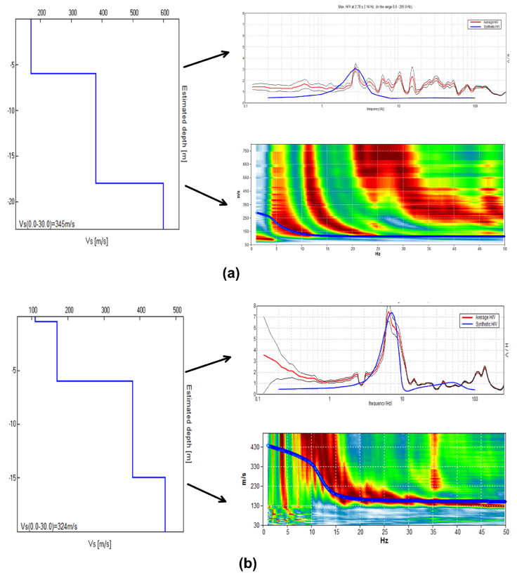
In order to validate the shear wave velocity profile obtained at these two sites from regression relation, seismic data has been collected using MASW and HVSR surveys at these sites. The joint inversion of HVSR and dispersion curve obtained from seismic data at each of these two sites is shown in Figure 12. Shear wave velocity profile obtained from joint inversion of seismic data and that from developed regression relation for the lithological unit has been compared in Figure 13. Root mean square error between shear wave velocity profile obtained from joint inversion of seismic data and developed regression relation at these two locations is 29 and 11 m/s respectively, which validates the applicability of the developed regression relation in this area.

Figure 13 Comparison of shear wave velocity profile obtained from joint inversion of seismic data and that from developed regression relation for different lithologic units. In this figure blue line indicates the shear wave profile obtained from developed relation and the red that from joint inversion of seismic data, respectively
One of the important seismic parameters that are used for the classification of foundation sites is the average shear wave velocity at 30 m depth which is commonly known as VS30. Site classification based on VS30 given by EUROCODE 8 is shown in Table 2. Table 2 shows the European site classification of Eurocode 8 which specifies the site type (A, B, C, D, E) according to the average shear wave velocities at 30 m depth.
Table 2 European seismic code classes of Eurocode 8 (European committee for standardization [CEN,2004])
| CLASS | EUROCODE 8 |
|---|---|
| A | >800 |
| B | 360-800 |
| C | 180-360 |
| D | <180 |
| E | Surface alluvium layer with Vs values of type C or D and thickness b/w 5 and 20 m, underlain by stiffer material of Vs > 800 m/s. |
The classification of sites BH 95 and BH 96 has been made based on VS30 obtained from both the regression relation and seismic survey. The estimate of VS30 from regression relation and seismic survey is given in Table 3. It is seen that VS30 obtained at these two sites from the seismic profile prepared using regression relation matches closely with that obtained from the seismic survey. The obtained VS30 at these stations from two different approaches classify these sites in Type C as per EUROCODE (CEN, 2004) classification. The comparison presented in Table 3 indicates that the developed regression relationship can be effectively used for the estimation of shear wave velocity profile and classification of rock in this part of Garhwal Himalaya.
Table 3 Comparison of VS30 value obtained from shear wave profiles from developed relation and that from joint inversion of seismic data, respectively
| SITE | VS30 (m/s) obtained from joint inversion of seismic data | VS30 (m/s) obtained from developed relation | Difference (m/s) |
|---|---|---|---|
| BH 95 | 345 (Type C) | 341 (Type C) | 4 |
| BH 96 | 324 (Type C) | 350 (Type C) | 26 |
Conclusions
In the present work, shear wave velocity structure has been estimated using both active and passive methods at a total of twenty-six sites in Garhwal Himalayas, India. In this work shear wave profiles from twenty-four sites have been used to prepare linear regression relation between shear wave velocities in different formations with respect to their depth of occurrence. In order to correctly identify various lithological units, lithologies from borehole data at each site have been used. Observed and calculated shear wave velocity from relation and seismic data is compared in terms of root mean square error. Root mean square error obtained for different lithological units varies from 5 to 28 m/s. In order to check the validity of regression relation two sites that have not been used for computing regression relation have been selected. Lithologs available at these sites are used for selecting regression relations of various lithological units. Shear wave velocity profile from joint inversion of H/V and MASW data at these sites is compared with that obtained from regression relation. Comparison of shear wave velocity profiles clearly shows that VS30 of shear wave velocity profile obtained from seismic experiment and regression relation falls in same EUROCODE 8 classification of the rock, thereby establishing the efficacy of developed relation in Garhwal Himalayas and thus is useful in contribution towards soil classification for zoning purposes and towards mitigation of region’s seismic risk.

