


 text new page (beta)
 English (pdf)
 Article in xml format
 Article references
 Send this article by e-mail
 Cited by SciELO
  Similars in
SciELO
Similars in
SciELO 
 Permalink
Introduction
El Mayor-Cucapah earthquake has provided an important opportunity to study about the geodynamics of the northwest region of Mexico (Fletcher et al., 2016), as spatial and tectonic geodesy (Wei et al., 2011). The use of GPS in seismology was first documented by Hirahara et al., (1994), Ge et al., (2000) and Nikolaidis et al., (2001), who demonstrate the potential of GPS as a seismological instrument. For instance, Larson et al., (2003) using GPS (1 Hz) achieved to observe the kinematic displacements of the Alaska Denali earthquake (Mw 7.9) in 2002, suggesting that GPS observations are crucial to study rupture processes. Miyazaki et al., (2004) compared displacements from GPS with the double integration of the acceleration records, finding a good correlation between both for the Tokachi-Oki earthquake (Mw 8.3, occurred in 2003). Blewitt et al., (2006) demonstrated the GPS ability to estimate the magnitude of a megathrust earthquake, using data from up to only a few minutes after earthquake initiation, as well as its high tsunamigenic potential for the Sumatra-Andaman earthquake (Mw 9.2-9.3) in 2004; whereas, Hung et al., (2017) shown that 5 Hz high-rate GPS observations is an optimal sampling rate for GPS seismology as observed for the Ruisi Taiwan earthquake occurred in 2013. Nowadays, broadband and/or strong-motion seismic instruments located with highrate GPS receivers are the best instrumental candidates to measure the complexity in the seismic source, rapid slip characterization of finite fault rupture and also for applications on early seismic warning systems (Melgar et al., 2013; Bock et al., 2011; Bock and Melgar, 2016).
Northern Baja California tectonics is primary dominated by right-lateral strike slip of ~50 mm/yr along southernmost San Andreas Fault system, between the Pacific and North American plates (Argus et al., 2010; DeMets et al., 2010) (Figure 1-inset). The El Mayor-Cucapah earthquake (32.278° N, 115.339° W; 4 km Depth; Mw 7.1; To=2010-04-04 22:40:40 UTC; RESNOM Database) of April 4, 2010, Mw 7.2, had a complex bidirectional rupture divided into two main domains from the epicentral zone located in the southeast corner of the Sierra Cucapah mountain range (Hauksson et al., 2010; Fletcher et al., 2014). The rupture in the northern section spread through the Cucapah mountains by several multiple faults-segments: Pescadores, Borrego, Paso Superior e Inferior. While in the southern section it extended through the Colorado River Delta, where it was possible to identify a new fault named Indiviso. The extent of the rupture was around 120 km (Figure 1) (González-García et al., 2010; Wei et al., 2011, Fletcher et al, 2014).
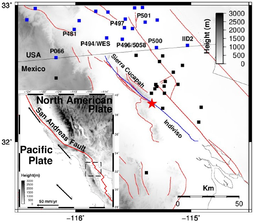
Figure 1 Tectonic setting of the north Baja California region, where the El Mayor-Cucapah earthquake occurred. The red star denotes the earthquake epicenter. Blue line denotes the surface rupture [Fialko et al., 2010] and red lines denote known active faults. Blue squares denote GPS continuous recording sites in USA during the earthquake occurrence and black squares are GPS temporal surveyed sites after the earthquake (González-Ortega et al., 2014). P494/WES and P496/5058 are colocated GPS and strong-motion instruments; as well as, P066, P481 P497, P50, P500 and IID2 are GPS stations used in the present study. Inset illustrates a broader tectonic setting of the study area. Black vectors shows the tectonic motion with respect to North American Plate.
The characterization of a seismic source depends primarily on the direction of propagation of the seismic waves, distribution of the rupture and the magnitude of the coseismic displacements (Hanks, 1981). One way to estimate earthquake source parameters (seismic moment, stress drop and source radius) is computing the Fast Fourier Transform (FFT) to the displacements in the far-field (Savage, 1972), and getting the spectral parameters (level at low frequencies, corner frequency and slope to high frequencies), to obtain the seismic moment (M0) (Brune, 1970), and then the moment magnitude (Mw) (Hanks and Kanamori, 1979) of an earthquake.
High-rate GPS (from 1-10 Hz) displacements has been proved very useful for monitoring long-period ground motion, moreover, the optimal combination of near-source GPS and seismic strong-motion data covers a broad spectrum of coseismic motion, from high frequencies to long periods (Bock and Melgar, 2016). Taking advantage of the availability of high-rate GPS records (5 Hz) nearby the seismic rupture of the El Mayor-Cucapah earthquake, the position ground motion was obtained, and then the results were compared with the double integration of acceleration data, for two sets of located (close to each other) GPS and strong-motion instruments. In the case of acceleration data a first order Butterworth filter was used within 0.10 - 50 Hz (Bendat and Piersol, 2011; Oppenheim and Shafer, 2011) in the frequency domain, while not for the GPS position. Finally, the earthquake seismic moment was estimated using a simple earthquake source model (Brune, 1970; Kumar et al., 2012) and moment magnitude was obtained following Hanks and Kanamori (1979).
Data and Methods
High-rate GPS (5Hz) data were used from the Plate Boundary Observatory GPS network (Figure 1), obtained through the University NAVSTAR Consortium (UNAVCO) and acceleration data from Southern California Earthquake Data Center (SCEDC), and Center for Engineering Strong Motion Data (CESMD) for the El Mayor-Cucapah earthquake.
The technique used to process the GPS data was Precise Point Positioning (PPP) with GIPSY-OASIS software (Zumberge et al., 1997; Kouba and Heroux 2001). PPP is a positioning technique that is based on precise position coordinates obtention for a single station without a reference station, using precise orbit products and clock corrections provided by the International GNSS Service (IGS) (Abdallah and Schwieger, 2014). This technique can be used for both kinematic and static GPS processing. To achieve centimeter-level accuracy estimates, several modeling effects must be taken into account, such as the atmospheric effects on the carrier phase, as well as terrestrial and oceanic tides (Heroux et al., 2001). Thus, from far-field displacements in the frequency domain, earthquake seismic moment and magnitude can be obtained (Hanks and Wyss, 1972; Johnson and McEvilly, 1974).
The simplest and widely used earthquake source models are those proposed by: Haskell (1964) and Brune (1970). In the Haskell's model, two corner frequencies
Thus the spectrum is parametrized by three factors, seismic moment Mo, raise time t d and rupture time t r (Stein and Wysession, 2003). The Brune's model has a single corner frequency, f c , that combines the effects of rise and rupture time. The amplitude spectrum corresponds to displacements observed in the far-field; however, it is also applicable for observations in the near-field as long as the source-receiver distance is greater than the wavelength of the seismic waves (Madariaga, 1989). In the present case, a wavelength of ~26 km is obtained when considering seismic wave velocity of 3.3 km/s (Fuis et al., 1982) and 8 s period of the first oscillation for P494 station (Figure 2).
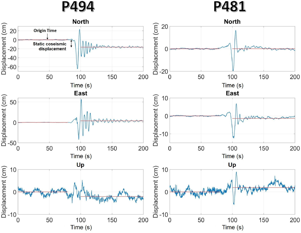
Figure 2 GPS position time series. Left column, GPS site P494, ~65 km from epicenter. Right column, GPS site P481, ~87 km from epicenter. Red lines indicate linear detrend removed before and after the S-wave arrival to estimate the static coseismic offsets.
One of the most important spectral parameter is the flat line-segment of the amplitude spectrum at low frequencies as proposed by Haskell (1964) and Brune (1970). This frequency line-segment is commonly referred as Ω0 , spectral level to low frequencies, from this parameter seismic moment is (Brune, 1970; Archuleta et al., 1982),
Where Ω0 is the line-segment at low frequencies,
Results
GPS position time series corresponding to the nearest sites to the earthquake rupture are shown in Figure 2. The kinematic displacement generated by the passage of the seismic waves can be observed, as well as the coseismic permanent displacement, derived from the surface motion of the El Mayor-Cucapah earthquake. Differences in amplitude and oscillation are due to the type of soil and epicentral distance. P494 is located ~65 km from the epicenter in the west Salton Sea basin; while P481 is ~87 km in the Peninsular Ranges. To estimate the coseismic displacements, the linear trend of the surperficial pre-arrival seismic wave was first calculated and then the entire record of the position time series. Subsequently, the mean of the oscillations of the pre-arrival and post-arrival segments was calculated, the difference between both segments corresponds to the static (permanent) coseismic displacement. In Table 1, the kinematic and static coseismic displacements for GPS sites processed in this study is presented.
Table 1 3D Coseismic displacements estimates from GPS position time series. Includes earthquake distance to GPS sites, peak-to-peak oscillation seismic wave motion, flat line segment amplitude value at low frequencies Ω0 , M 0 and M w .
| GPS site |
Lat. | Long. | Epicentral distance (km) |
Kinematic peak to peak oscillation, north (cm) |
Kinematic peak to peak oscillation, east (cm) |
Kinematic peak to peak oscillation, Up (cm) |
Static coseismic north (cm) |
Static coseismic east (cm) |
Static coseismic Up (cm) |
Ω0 (cm-s) |
M
o
(dyne-cm) 1×1026 |
M w |
|---|---|---|---|---|---|---|---|---|---|---|---|---|
| P494 | 32.760 | -115.732 | 65 | 90 | 100 | 10 | -18 | 4 | ~ -1 | 160 | 10.8 | 7.32 |
| P496 | 32.751 | -115.596 | 58 | 60 | 95 | 24 | -17 | ~2 | ~0 | 150 | 9.0 | 7.27 |
| P497 | 32.835 | -115.577 | 67 | 40 | 60 | 15 | -9 | ~1 | ~1 | 125 | 8.7 | 7.26 |
| P501 | 32.876 | -115.398 | 67 | 45 | 36 | 10 | -5 | ~2 | ~1 | 137 | 9.5 | 7.29 |
| P500 | 32.690 | -115.300 | 46 | 26 | 30 | 12 | -4 | 5 | ~0 | 93 | 4.4 | 7.06 |
| IID2 | 32.706 | -115.032 | 54 | 16 | 21 | NA | ~ -2 | 3 | ~0 | 77 | 4.3 | 7.06 |
| P481 | 32.822 | -116.012 | 87 | 36 | 20 | 15 | ~ -2 | ~ -1 | ~0 | 74 | 6.7 | 7.18 |
| P066 | 32.617 | -116.170 | 90 | 16 | 11 | 13 | ~0 | -7 | ~0 | 51 | 4.8 | 7.08 |
GPS position time series were compared with the displacement series obtained from the double integration of the accelerometer records from WES and 5058 accelerograph stations, located at <1 km from GPS sites P494 and P496, respectively (Figure 3). Horizontal components show alignment in phase and similarity in amplitudes (see inset plots). For strong-motion data several tests to find the frequency range and order for the Butterworth filter were performed. First-order Butterworth bandpass filter was selected, from 0.08 and 0.20 to Nyquist frequency for WES and 5058 respectively. This type of filter allows to improve the position of the time series and to carry out the comparison with GPS position time series. High order Butterworth filters tend to generate biases in position baseline and cause distortions [Oppenheim and Schafer, 2011].
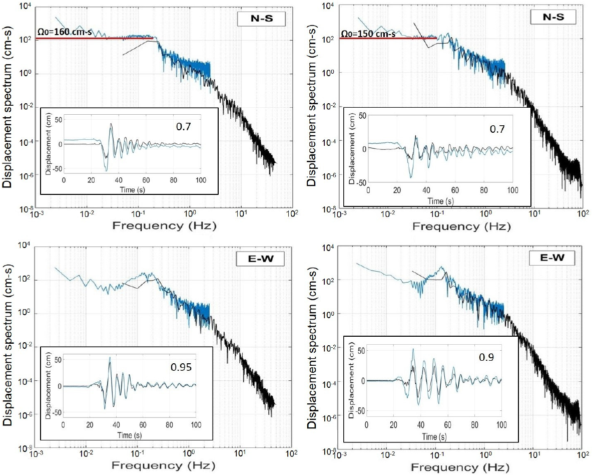
Figure 3 Displacement spectrum comparisons from collocated strong motion (black) and high-rate GPS (blue). Left column, horizontal displacement spectrum at P494-GPS and WES accelerograph station. Right column, horizontal displacement spectrum at P496-GPS and 5058 accelerograph station. Red horizontal lines indicate Ω0 value. Insets show comparison between GPS and integrated (from strong-motion) time series displacement and corresponding cross-correlation values estimate.
To compare the kinematic GPS displacements and double integrated accelerogram data, a normalized cross-correlation was used. In general, correlation values are better in the east-west (>0.90) than north-south (>0.70), due to the smaller kinematic coseismic displacement in the east-west direction. Consequences of seismic filtering tends to diminish the amplitudes of the displacement series obtained from accelerogram double integration data when compared to those obtained with GPS. Static coseismic displacements are not observable in strong-motion due to broadband limitation but in GPS these are clearly captured.
Figure 3 shows horizontal GPS and strong-motion source spectra comparison for P494-GPS and WES, as well as, P496-GPS and 5058. With GPS spectra, the amplitude at low frequencies Ω0 is easily identified. After a value of ~0.2Hz, amplitudes decay at f -2 as frequency increases up to where GPS spectra turns constant. At this point, seismic oscillations with spectral amplitudes of ~2cm-s associated with frequency values ~1Hz (periods ≥ 1 s for 5Hz GPS sampling rate), are not detectable with GPS. On the other hand, with strong-motion displacement spectra, two corner frequencies at ~0.2Hz and ~3Hz can be identified. For frequencies >3Hz amplitude decay as f -4. These amplitude decays are related to attenuation and site effects [Shearer, 1999].
Seismic moment (M o ) and moment magnitude (M w) of the El Mayor-Cucapah earthquake is M o = 7.3±3.5×1026 dyne-cm, M w = 7.19±0.13 using GPS spectra (Table 1), and Mo = 6.4±0.07×1026 dyne-cm, M w = 7.14±0.01, using WES and 5058 strong-motion data spectra. These values are similar to estimates obtained from seismic and geodetic data inversion M o = 9.9×1026 dyne-cm, M w = 7.26 [Wei et al., 2011] and from field measurements of M o = 7.2×1026 dyne-cm, M w = 7.17 [Fletcher et al., 2014].
Figure 4 shows the El Mayor-Cucapah static coseismic horizontal displacements. The maximum horizontal static coseismic displacement is ~1.16 m, in the N137°E direction, ~8 km from the epicenter, in the southeastern part of the Sierra Cucapah, and the maximum vertical displacement is ~-0.64 m. The displacement pattern, clearly observed in the northeast is consistent with a right-lateral focal mechanism of The El Mayor- Cucapah earthquake (González-Ortega et al., 2014). These authors, estimated earthquake moment magnitude using dislocation inversion methods from a finite coseismic slip model composed of several fault segments using GPS and InSAR static displacements in a homogeneous (Fialko et al., 2010) and in a layered earth structure [Huang et al., 2016].
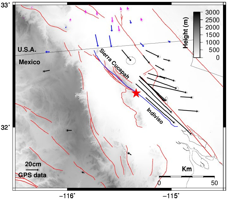
Figure 4 GPS horizontal coseismic displacements from El Mayor-Cucapah earthquake. Blue vectors are estimates obtained in this study. Black are displacements from Gonzalez-Ortega (2014), and magenta are from GPS Explorer Data Products (http://geodemo-c.ucsd.edu). The red star denotes the earthquake epicenter. Blue line denotes the surface rupture [Fialko et al., 2010] and red lines denote known active faults.
Discussion
Zheng et al., (2012), also used high-rate GPS data with the aim of carrying out the seismotectonics analysis of El Mayor-Cucapah earthquake with different methodology as in this work. They used the Cut and Paste method (CAP) developed by Zhu and Helmberger (1996), which allows separating the P n and surface waves independently, not requiring an accurate crustal velocity model or a high number of stations, but a good azimuthal coverage for the focal mechanism inversion and earthquake magnitude. Also, Allen and Ziv,(2011), reprocessed in a simulated real-time high-rate GPS static displacement data, to estimate earthquake magnitude via static slip inversion, using preliminary earthquake hypocenter from seismic data and a catalog of active faults, for the purpose of earthquake early warning system test in southern California.
Differences between Zheng et al., (2012), and the present work lies in the GPS data processing; while we used the PPP technique, they used the Double Differences (DD). For the DD technique (Herring et al., 2015) it is necessary to have a reference station, which must be located at a distance far enough not to be affected by seismic waves, but close enough to act as reference station which guarantees the same satellites observation of the sites of interest. Such condition is not required with PPP technique, as it uses precise GPS orbit and clock data products with centimeter accuracy. Although the methodology used in Zheng et al., (2012) and the present one differ in estimating GPS time series and seismic moment, in general, position time series and moment magnitude results are very similar and confirm earlier studies using GPS high-rate data from El Mayor-Cucapah earthquake (Allen and Ziv, 2011; Bock et al., 2011).
With high-rate GPS spectral analysis, amplitude at low frequencies is clear to identify in contrast to accelerogram data. This flat low frequency section is associated with large displacement amplitudes generated by the passage of surperficial seismic waves (Udias, 1989). Thus, estimates of M o and M w can have a greater degree of certainty with GPS data than with accelerometer records, which can be of crucial importance for estimating major earthquake magnitude in real time (Blewitt et al., 2006; Bock and Melgar, 2016). According to the present results, average Ω0 value with GPS data is 115±4 cm-s, while with accelerogram data is 90±8 cm-s. However, as GPS is sampled at 5 Hz, for frequencies >2.5 Hz (Nyquist frequency) GPS is unable to observe spectral displacements below 2 cm-s, which does not happen with the acceleration records. This highlights the importance of the complementarity between both instruments, closely located GPS and strong-motion, for near field displacements earthquake studies.
Conclusion
High-rate (5 Hz) kinematic GPS position time series of the El Mayor-Cucapah earthquake were studied and compared to the displacement series obtained from the double integration of strong-motion data. The comparison shows good agreement in terms of cross-correlation, for P494-GPS and WES, and, P496-GPS and 5058, instruments at ~70 km from epicenter. Kinematic GPS data at low frequencies, associated with large spectrum displacements, help to clearly identify the flat line segment amplitude better than accelerogram data, and thus using a simple earthquake source model the earthquake seismic moment, Mo=7.3±3.5×1026 dyne-cm, Mw=7.19±0.13 could be estimated, similar to Mw 7.2 as previously reported using other methodologies. Static coseismic displacements are very difficult to obtain from accelerogram data, however with GPS data, these are easily obtained and consistent with the right-lateral strike-slip mechanism of the El Mayor-Cucapah earthquake.
Data and Resources
High-rate GPS data can be found at UNAVCO, ftp://data-out.unavco.org/pub/highrate/5-Hz/rinex/ (last accessed April 2018). Coseismic displacements from the northern side of the El Mayor-Cucapah rupture can be found at GPS Explorer, http://geodemo-c.ucsd.edu (last accessed April 2018). Accelerometric data can be found at SCEDC, http://scedc.caltech.edu/research-tools/waveform.html (last accessed April 2018) and CESMD, https://www.strongmotioncenter.org/cgi-bin/CESMD/search_options.pl (last accessed April 2018). Map figures were generated by Generic Mapping Tool (GMT) software [Wessel et al., 2013].

