Introduction

Mathematical models occurring in science and engineering, lead to systems of partial differential equations (PDEs) (^{Herrera and Pinder, 2012}), whose solution methods are based on the computational processing of large-scale algebraic systems and the advance of many areas, particularly Earth Sciences, depends on the application of the most powerful computational hardware to them (^{President's Information Technology Advisoty Committee, 2005}).

Parallel computing is outstanding among the new computational tools, especially at present when further increases in hardware speed apparently have reached insurmountable barriers.

As it is well known, the main difficulties of parallel computing are associated with the coordination of the many processors that carry out the different tasks and the information- transmission. Ideally, given a task, these difficulties disappear when such 'a task is carried out with the processors working independently of each other'. We refer to this latter condition as the 'paradigm of parallel- computing software'.

The emergence of parallel computing prompted on the part of the computational-modeling community a continued and systematic effort with the purpose of harnessing it for the endeavor of solving the mathematical models of scientific and engineering systems. Very early after such an effort began, it was recognized that domain decomposition methods (DDM) were the most effective technique for applying parallel computing to the solution of partial differential equations (DDM Organization 1988-2014), since such an approach drastically simplifies the coordination of the many processors that carry out the different tasks and also reduces very much the requirements of information-transmission between them (^{Toselli and Widlund, 2005}) (^{Farhat et al., 2000}).

When a DDM is applied, firstly a discretization of the mathematical model is carried out in a fine-mesh and, afterwards, a coarse-mesh is introduced, which properly constitutes the domain-decomposition. The 'DDM-paradigm', a paradigm for domain decomposition methods concomitant with the paradigm of parallel-computing software (^{Herrera et al., 2014}), consists in 'obtaining the global solution by solving local problems exclusively' (a local problem is one defined separately in a subdomain of the coarse-mesh). Stated in a simplistic manner, the basic idea is that, when the DDM-paradigm is satisfied, full parallelization can be achieved by assigning each subdomain to a different processor.

When intensive DDM research began much attention was given to overlapping DDMs, but soon after attention shifted to non-overlapping DDMs. When the DDM-paradigm is taken into account, this evolution seems natural because it is easier to uncouple the local problems when the subdomains do not overlap. However, even in this kind of methods different subdomains are linked by interface nodes that are shared by several subdomains and, therefore, non- overlapping DDMs are actually overlapping when seen from the perspective of the nodes used in the discretization. So, a more thorough uncoupling of the local problems and significant computational advantages should be expected if it were possible to carry out the discretization of the differential equations in a 'non-overlapping system of nodes' (^{Herrera et al., 2014}); i.e., a set of nodes with the property that each one of them belongs to one and only one subdomain of the coarse-mesh (this is the mesh that constitutes a domain decomposition). In (^{Herrera et al., 2014}), as in what follows, discretization methods that fulfill these conditions are referred to as non- overlapping discretizations.

In a line of research, which this paper belongs to, I. Herrera and co-workers addressed this problem and to cope with it have developed a framework -the 'DVS- framework'- thoroughly formulated using a non-overlapping discretization of the original partial differential equations. Due to the properties of non-overlapping discretizations in such algorithms the links between different processors are very much relaxed, and also the required information-transmission between them is reduced. Such properties, as well as preliminary analysis of the algorithms, indicate that they should be extremely adequate to program the treatment of partial differential equations occurring in science and engineering models by the highly parallelized hardware of today. Although the DVS-algorithms have already been significantly developed and some examples have been previously treated (^{Herrera et al., 2014} and ^{Carrillo-Ledesma et al., 2013}), up to now no software that took full advantage of the DVS-algorithms had been developed. Clearly, to profit fully from such advances it is essential to develop software, carefully coded, which permit applying effectively the DVS-algorithms to problems of interest in science and engineering. As a further contribution to these advances, in this paper, for the first time we present and test software of such characteristics.

Overview of DVS-software

The derived-vector-space framework (DVS- framework) deals with the matrix that is obtained after the partial differential equation (PDE), or system of such equations, has been discretized by means of a standard discretization procedure (i.e., an overlapping discretization). The resulting discrete system of equations is referred to as the original-system.

The DVS-procedures follow the next steps:

1. The partial differential equation, or system of such equations, is discretized by any standard method that satisfies the axioms of the theory (here stated in section how to build non-overlapping discretizations) in a mesh -called the fine-mesh- to obtain a discrete problem that is written as

(2.1)

This is called the original-problem, while the nodes of the fine-mesh are called original-nodes. The notation X^ will be used for the whole set of original-nodes; any function defined on the set X^ by definition is an original-vector. Finally, the notation W^ will be used for the linear space spanned by the original-vectors, which in turn is called original-vector space;

2. A coarse-mesh is introduced, which constitutes a non-overlapping decomposition of the problem-domain. The system of original- nodes turns out to be overlapping with respect to the coarse-mesh;

3. A system of non-overlapping nodes (the derived-nodes), denoted by X, is constructed applying the procedure explained in previous articles (see also preliminary notions and notations). The functions defined in the whole set X are by definition the derived-vectors and the notation W is used for the whole linear space of derived-vectors, which constitutes the derived-vector space;

4. The theory of the DVS-framework supplies a formula that permits transforming the original-discretization into a non-overlapping discretization. Applying this formula the non-overlapping discretization is obtained. This is another discrete formulation that is equivalent to the original-problem, except that it constitutes a non-overlapping discretization; and

5. Thereafter, each one of the coarse-mesh subdomains is assigned to a different processor and the code is programmed separately in each one of the processors.

The theoretical DVS-framework is very elegant; in it, the algebraic operations can be carried out systematically and with great simplicity. Furthermore, many simplifying algebraic results have been obtained in previous work (^{Herrera et al., 2014} and ^{Herrera and Yates, 2011}). To optimize the communications and processing time a purely algebraic critical- route is defined, which profits much from such algebraic results previously obtained. Then, this algebraic critical-route is transformed into a computational code using C++ and several well-established computational techniques such as MPI.

Following the steps indicated above, in the present paper software for problems of isotropic elastic solids in equilibrium has been developed and tested experimentally. The high parallelization efficiency of the software so obtained has been verified experimentally. To be specific, only the DVS-BDDC algorithm has been implemented for this problem. However, by simple combinations of the routines already developed the other DVS-algorithms can be implemented.

The standard discretization

Following the steps succinctly described in overview of DVS-software, software that constitutes a tool for effectively applying massively parallel hardware to isotropic elastic solids in equilibrium was constructed. In particular, it permits to treat the following boundary value problem (BVP):

(3.1)

Subjected to the Dirichlet boundary conditions:

(3.2)

By simple modifications of the code, other boundary conditions can also be accommodated.

The software that we have developed treats in parallel the discrete system of linear equations that is obtained when the standard discretization method used to obtain the original discretization of the Dirichlet BVP defined by Eqs. (3.1) and (3.2) is the finite element method (FEM). In particular, it was obtained applying the well-known variational principle:

(3.3)

with linear functions.

Such system of equations can be written as

(3.4)

Here, it is understood that the vectors U and F, are functions defined on the whole set of original-nodes of the mesh used in the FEM discretization, whose values at each node are 3-D vectors. They can be written as . As for the matrix the notation

(3.5)

is adopted. Above, the range of p and q is the whole set of original-nodes, while i and j may take any of the values 1, 2, 3.

Preliminary notions and notations

The DVS-approach is based on non-overlapping discretizations, which were introduced during its development (^{Herrera et al., 2014}). A discretization is non-overlapping when it is based on a system of nodes that is non- overlapping; to distinguish the nodes of such a system from the original-nodes, they are called derived-nodes. In turn, a system of nodes is non-overlapping, with respect to a coarse- mesh (or, domain-decomposition), if each one of them belongs to one and only one of the domain-decomposition subdomains. In the general DVS-framework, the derived-vector space (DVS) is constituted by the whole linear space of functions whose domain is the total set of derived-nodes and take values in Rn. In the present paper, where problems of elasticity that are governed by a system of three PDEs are treated, we take n = 3. Usually, when the basic mathematical model is governed by a single differential equation, n is chosen to be equal to 1.

Generally, when the coarse-mesh is introduced some of the nodes of the fine-mesh fall in the closures of more than one subdomain of the coarse-mesh. When that is the case, a general procedure for transforming such an overlapping set of nodes into a non-overlapping one was introduced in previous papers (see ^{Herrera et al., 2014}). Such a procedure consists in dividing each original-node into as many pieces as subdomains it belongs to, and then allocating one and only one of such pieces to each one of the subdomains. For a case in which the coarse-mesh consists of only four subdomains, this process is schematically illustrated in Figures 1 to ⁴.

Figures 1 to 4 

Then, the final result is the system of non- overlapping nodes shown in Figure 4. Each one of the non-overlapping nodes is uniquely identified by the pair (p, α), where p is the original-node it comes from and α is the subdomain it belongs to. Using this notation, for each fixed β = 1, ..., E, it is useful to define X^β ⊂ X as follows: The derived node (p, α) belongs to X^β, if and only if, α = β.

In what follows, the family of subsets{X¹,..., X^E} just defined will be referred to as the non-overlapping decomposition of the set of derived-nodes. This because this family of subsets of X possesses the following property:

(4.1)

An important property implied by Eq. (4.1) is that the derived-vector space, W, is the direct-sum of the following family of subspaces of W: { W¹ , ..., W^E }; i.e.,

(4.2)

Here, we have written

(4.3)

The notation W(X^α), introduced previously (see, for example ^{Herrera et al., 2014}), is here used to represent the linear subspace of W whose vectors vanish at every derived- node that does not belong to X^α. An important implication, very useful for developing codes in parallel, is that every derived-vector w_∈W can be written uniquely in the form

(4.4)

As it is customary in DDM developments, in the DVS-approach a classification of the nodes used is introduced. We list next the most relevant subsets of X used in what follows:

Also, we observe that each one of the following set-families are disjoint: {I, Г }, {I, π, ∆}, {∏, ∆} and {∑, π}, while

(4.6)

Next, we highlight some of most important notation and nomenclature used in the DVS- framework; for further details the reader is referred to previous works of this line of research (in particular (^{Herrera et al., 2014}), where additional references are given). When considering any given derived-node, which is identified by the pair of numbers (p, α), the natural number p (which corresponds to an original-node) is called the 'ancestor' of the derived-node, while α (which ranges from 1 to E) identifies the subdomain it belongs to. Furthermore, for every original-node p∈X^, the notation Z(p)⊂X will be used to represent the set of derived-nodes that derived from it. Then, the 'multiplicity of p', m(p), is the cardinality of Z(p).

We observe that the multiplicity of p is defined as a property of each original-node, p. There is another kind of multiplicity that is used in the DVS-framework, which is defined as a property of each pair (p, q) of original- nodes and is also used in the DVS-framework theory. To introduce it, we define

(4.7)

Then, the multiplicity of the pair (p, q) -written as m(p, q)- is defined to be

(4.8)

When u is a derived-vector, so that u is a function defined on X, u(p, α) stands for the value of u at the derived-node (p, α). In particular, in applications of the DVS- framework to elasticity problems, those values are -vectors and the real-number u(p, α, i) - i = 1, 2, 3- will be the i−th component of the vector u(p, α). The derived-vector space is supplied with an inner product, the 'Euclidean inner-product', which using the above notation for every pair of derived-vectors, u and w, is defined by

(4.9)

For the parallelization of the algorithms the relation

(4.10)

will be useful, because the vector-components corresponding to different subdomains will be handled by different processors when implementing them.

Let p∈X^ be an original-node and u∈W a derived-vector. Then, u∈W is said to be 'continuous at p' when u(p, α) is independent of α, and it is said to be of 'zero-average at p' when

(4.11)

When the corresponding properties are satisfied for every p∈ X^, the derived-vector u is simply said to be 'continuous' or 'zero- average'. The linear subspaces W₁₂ and W₁₁ of W, are constituted by the continuous and the zero-average vectors of W, respectively. These two subspaces are orthogonal complements of each other. The matrices and are the orthogonal projections on W₁₂ and on W₁₁ , respectively. They satisfy:

(4.12)

where is the identity matrix. For any w∈W, the explicit evaluation of v ≡ is given by:

(4.13)

Using this equation, the evaluation of is also straight forward, since Eq. (4.12) implies

(4.14)

The natural injection of into W, written as R:→W, is defined for every by

(4.15)

When necessarily. We observe that = W₁₂ . Furthermore, it can be seen that R has a unique inverse in W₁₂; i.e., R^-1 : W → is well-defined.

How to build non-overlapping discretizations

This Section explains how to transform a standard (overlapping) discretization into a non-overlapping discretization. The DVS procedure here explained permits transforming an overlapping discretization into a non- overlapping discretizations and yields directly preconditioned algorithms that are subjected to constraints. It can be applied whenever the following basic assumption is fulfilled:

(5.1)

Here, the symbol ⇒ stands for the logical implication and it is understood that M is the matrix occurring in Eq. (2.1).

We define the matrix ̳α' by its action on any vector of W: when u∈W, we have

(5.2)

We observe that the action of can be carried out by applying the operator at the primal-nodes exclusively. Then, we define the 'constrained space' by

(5.3)

Clearly, W^r⊂W is a linear subspace of W and for any u∈W, u is the projection of u, on W^r.

Now, we define

(5.4)

For γ = 1, ..., E, we define the matrices

(5.5)

Next, we define the matrices:

(5.6)

and

(5.7)

Then, we define

(5.8)

The following result was shown in previous papers (^{Herrera et al., 2014}):

Theorem 5.1.- Let U∈Ŵ and u∈W be related by u=RU, while f ∈W₁₂ is defined by

(5.9)

Here, is a diagonal matrix that transforms into itself, whose diagonal-values are m(p), while here its inverse is denoted by . Then, the discretized version of static elasticity of Eq.: (3.4):

(5.10)

is fulfilled, if and only if

(5.11)

Proof.- See for example (^{Herrera et al., 2014}).

The preconditioned DVS-algorithms with constraints

There are four DVS-algorithms (^{Herrera et al., 2014}), and two of them are the DVS-BDDC and the DVS- FETI-DP. These are DVS versions of the well-known BDDC (^{Dohrmann, 2003}), (^{Mandel et al., 2005}) and FETI-DP (^{Farhat and Roux, 1991}), (Farhat et al., 2000). As for the other two, nothing similar had been reported in the literature prior to the publication of the DVS-algorithms. By now, it is well known that BDDC and FETI-DP are closely related and the same can be said of the whole group of four DVS-algorithms.

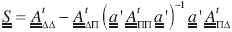
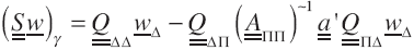
The DVS-Schur-complement is defined by

(6.1)

We also define

(6.2)

Then, writing u ≡ u _∏+ u _∆ it has been shown (^{Herrera et al., 2014}) that Eq. (5.11) is fulfilled if and only if

(6.3)

and

(6.4)

The general strategy followed in the DVS approach, is to find u _∆ ∈W(∆) first and then apply Eq. (6.4) to obtain the remaining part, u _∏ ∈W(∏), of u. For this strategy to be effective it is essential that the application of be computationally cheap. Different DVS- algorithms are derived by seeking different pieces of information such that u _∆ ∈W(∆) can be derived from it in a computationally-cheap

manner. In particular, the four DVS-algorithms mentioned before seek for: and respectively. Drawing from (^{Herrera et al., 2014}), they are here listed.

The DVS-BDDC algorithm

This algorithm seeks for u _∆ . It is:

(6.5)

The DVS-primal-algorithm

We set and the algorithm consists in searching for a function v _∆ ∈W_∆ , which fulfills:

(6.6)

Once v _∆ ∈W(∆) has been obtained, then

(6.7)

The DVS-feti-dp algorithm

This algorithm seeks for . Thus, the algorithm is: "Given such that

(6.8)

Once λ∈W_∆ has been obtained, is given by:

(6.9)

The DVS-dual-algorithm

In this case one seeks for using the relation:

(6.10)

Once μ∈W(∆) has been obtained, u _∆∈W(∆) is given by:

(6.11)

The elementary pieces of DVS-software

All the DVS-algorithms are iterative algorithms and can be implemented with recourse to Conjugate Gradient Method (CGM), when the matrix is definite and symmetric, as is the case of elasticity problems here considered, or some other iterative procedure such as GMRES, when that is not the case. At each iteration step, depending on the DVS-algorithm that is applied, one has to compute the action on an arbitrary derived-vector of one of the following matrices: . In turn, such matrices are different permutations of Thus, a code for implementing any of the DVS-algorithms can be easily developed when codes for carrying out the action of each one of such matrices are already available.

To produce such codes will be the goal of the next Section, while the remaining of this one is devoted to obtain some auxiliary results that will be used there and were previously presented in (^{Herrera et al., 2014}). The first one of such results is:

(7.1)

The second one is: When w∈W, the following identity holds

(7.2)

Here the notation stands for the component on .

The third and fourth results required refer to the pseudo-inverses that occur in Eqs. (7.1) and (7.2). They are:

Let w∈W^r(∏) and then

(7.3)

together with

(7.4)

Let w∈W^r and then

(7.5)

together with

(7.6)

These two results permit applying iterative algorithms, in which the CGM is used, when the actions of and respectively, are computed.

Construction of the DVS-software

All the DVS-algorithms presented in the Section on the preconditioned DVS-algorithms with constraints are iterative, as is the case with most DDM algorithms, and to implement them it is only necessary to develop parallelized codes capable of computing the action of each one of the matrices on an arbitrary derived-vector, as it was foreseen in (^{Herrera et al., 2014}).

In the code here reported, all system-of- equations' solutions that were non-local were obtained with the help of the CGM algorithm. Due to this fact, actually the following subprograms were required: and . Furthermore, the application of

(8.1)

requires to compute the action of which is non-local. Thus, an efficient subprogram to carry-out this operation efficiently in parallel was required and was developed.

The communications required by DVS- algorithms are very easy to analyze. Indeed, when a different processor is allocated to each one of the coarse-mesh subdomains (i.e., to the subsets of derived-nodes, X^α, α = 1, ..., E, of the non-overlapping partition of X) -as it was done in the work here reported- transmission of information between different processors occurs only when the global Euclidean inner- product is computed, or either the matrix or the matrix is applied. Furthermore, in these operations the amount of information transmitted is very small.

In a first tentative version of the software, a master-processor was also used. However, using such a master-processor as a communications center is very time-costly and when the master-processor is not used as a communications center the work done by it is so small that it can be eliminated easily. When this is done, the performance of the DVS-algorithm became extremely good as it is explained and discussed in the Section on Numerical Results.

Only the DVS-BDDC algorithm was implemented. Although the implementation of the other three DVS-algorithms is very similar, and their expected parallel efficiency as well, their implementation would have taken additional time and effort that we preferred to save for future work.

Construction of the local DVS-software

A fundamental property of as defined by Eq. (5.7) is that it is block-diagonal, in which each one of the blocks is for each α = 1, ..., E, is a linear-transformation of Wα into itself. This property simplifies very much the parallelization of the codes to implement the DVS-algorithms.

To this end, each one of the subsets X^α of the non-overlapping decomposition of X, is assigned to a different processor and the set of processors is numbered accordingly. The fact that every vector w∈W can be written in a unique manner as

(9.1)

is used for this purpose. The processor γ handles only the w _γ component of every vector w∈W. Then, all the operations of the processor γ transform w _γ into a vector that also belongs to W ^γ ; even the operators and transform w _γ into a vector of W ^γ , except that and require information from of a few neighboring processors. However, it is important to make sure that such information be updated at the time it is gathered.

When evaluating the action on a vector of any of the matrices considered, processor γ will be responsible of constructing the g component of such a vector; in particular, depending on the matrix that is being applied. In what follows it is assumed that, from the start, the nodes of the set X^γ have been classified into Ι: internal, π: primal, and ∆: dual. Other node-classes of X^γ that will be considered are: ∏: extended-primal, and ∑: extended-dual. Without any further notice, the following relation will also be used:

(9.2)

The application of , and ̳j

To start with, we evaluate when w∈ W^γ . As it will be seen, the application of ̳α to any vector of W^γ requires exchange of information between processor γ and other processors. Indeed, recalling Eq. (4.13) we have

(9.3)

Thus, this operation requires information from the processors that possess derived-nodes belonging to Z(p); therefore, its computation involves communications between different processors, which may slow the processing. In view of Eq. (9.3), it is clear that except for this exchange of information, the evaluation of , is very simple. Once ,has been obtained, the relation , can be used to compute the action of . As for the action of , we recall that is obtained when the application of is restricted to primal-nodes.

Before going ahead, some final comments are in order. The application of , and hence that of , also requires transmission of information between the processors. Thus, for enhancing the efficiency of the codes it is essential that the application procedures be designed with great care. As it will be seen, with a few exceptions, all the exchange of information required when the DVS-algorithms are implemented is when the transformations and are applied.

The DVS-software for and ^~1

It should be observed that in view of the definition of the matrix and the submatrices occurring in the following decomposition:

(9.4)

for any they transform vectors of W(X^γ) into vectors of W(X^γ). Therefore, the local matrix Q is defined to be

(9.5)

where is the matrix defined in how to build non-overlapping discretizations, by Eq. (5.6). In this equation the index γ is omitted in the definition of , because γ is kept fixed. Due to the comments already made, it is clear that is a well-defined linear transformation of W^γ into itself. In particular, when w ^γ∈ W^γ , the computation of can be carried out in an autonomous manner, at processor γ, without exchange of information with other processors. This is a fundamental difference with , and , and implies that at each processor either the matrix is constructed, or internal software capable of evaluating its action on any vector of W^γ is made available.

In view of Eq. (9.4), the matrix will be written in two forms

(9.6)

The following expressions, which are clear in view of Eq. (9.6), will be used in the sequel:

(9.7)

Here:

(9.8)

and

(9.9)

A. The Local DVS-software for S

Let w_∆ ∈W, and recall Eq. (7.1); then:

(9.10)

In this equation the meaning of the terms and are clear since both and are well defined linear transformations of W^γ into itself. Something similar happens when the operator is applied to , since this is also a global linear transformation. It must also be understood that, when it is applied, the local vector has already been stored at processor g and at each one of the other processors. Due to the global character of the operator special software was developed for it.

A.1. The local DVS-software for (̳A _∏∏ )^~1

The local software that was developed is based on the next formula:

"Let w_∏∈W^r(∏) and v_∏ = w_∏ , then

(9.11)

together with

(9.12)

To apply this formula iteratively, at each processor γ it was necessary to develop local software capable of carrying out the following operations:

(9.13)

and, once convergence has been achieved, the following autonomous operation is carried out:

(9.14)

We see here that except for all the linear transformations involved are autonomous and can be expressed by means of local matrices defined in each processor. In the DVS-software that is the subject of this paper, such matrices were not constructed but we recognize that in some problems such an option may be more competitive,

B. The Local DVS-Software for ^~1

The local software that was developed is based on the next formula: "When w_∆ ∈W(∆), then

(9.15)

Therefore, if v∈ W^r is defined by the condition and it is written in the form v= v _I +v _∆ +v _π, then .A more explicit form of the condition v∈W^r is jv_π = 0. This latter condition together with the equation gives rise to a global problem whose solution, in the parallel software we have developed, was based on the iterative scheme:

"Let w _∆ ∈W(∆) and, then at processor γ:

(9.16)

Once v _π has been obtained, v _∆ is given by

(9.7)

At processor γ that is being considered, Eqs. (9.16) and (9.17) are:

(9.18)

and

(9.19)

respectively.

C. Applications of the Conjugate Gradient Method (CGM)

There are three main instances in which CGM was applied: i) to invert , ii) to invert ; iii) to solve iteratively the global equation -such equation may be: either Eq. (6.5), Eq. (6.6), Eq. (6.8) or Eq. (6.10), depending on the DVS-algorithm that is applied-. Furthermore, it should be mentioned that the inverses of the local-matrices: and can either be obtained by direct or by iterative methods; in the DVS-software here reported, this latter option was chosen and CGM was also applied at that level.

Numerical Results

In the numerical experiments that were carried out to test the DVS-software, the boundary- value problem for static elasticity introduced in the standar discretization was treated. In this paper only the DVS-BDDC algorithm has been tested. Work is underway to test the other DVS-algorithms, albeit similar results are expected for them. The elastic material was assumed to be homogeneous;π so, the Lamé parameters were assumed to be constant and their values were taken to be

These values correspond to a class of cast iron (for further details about such a material see, http://en.wikipedia.org/wiki/Poisson's_ratio) whose Young modulus, E, and Poison ratio, v, are:

The domain Ω⊂ R³ that the homogeneous- isotropic linearly-elastic solid considered occupies is a unitary cube. The boundary-value problem considered is a Dirichlet problem, with homogeneous boundary conditions, whose exact solution is:

(10.1)

The fine-mesh that was introduced consisted of (193)³ = 7,189,057 cubes, which yielded (194)³ = 7,301,384 original-nodes.

The coarse-mesh consisted of a family of subdomains {Ω₁, ..., Ω_E}, whose interfaces constitute the internal-boundary Г. The number E of subdomains was varied taking successively the values 8, 27, 64, 125, 216, 343, 512 and so on up to 2,744. The total number of derived-nodes and corresponding number of degrees-of-freedom are around 7.5 x 10⁶ and 2.5 x 10⁶, respectively. The constraints that were imposed consisted of continuity at primal-nodes; in every one of the numerical experiments all the nodes located at edges and vertices of the coarse mesh were taken as primal-nodes. In this manner, the total number of primal-nodes varied from a minimum of 583 to a maximum of 94,471. Thereby, it should be mentioned that these conditions granted that at each one of the numerical experiments the matrix was positive definite and possessed a well-defined inverse.

All the codes were developed in C++ and MPI was used. The computations were performed at the Mitzli Supercomputer of the National Autonomous University of Mexico (UNAM), operated by the DGTIC. All calculations were carried out in a 314-node cluster with 8 processors per node. The cluster consists 2.6 GHz Intel Xeon Sandy Bridge E5- 2670 processors with 48 GB of RAM.

As it was exhibited in the analysis of the operations, the transmission of information between different processors exclusively occurs when the average-operators and are applied. In a first version of the software reported in the present paper such exchange of information was carried out through a master-processor, which is time expensive. However, the efficiency of the software (as a parallelization tool) improved very much when the participation of the master-processor in the communication and exchange of information process was avoided. In its new version, the master-processor was eliminated altogether. A Table summarizing the numerical results follows.

It should be noticed that the computational efficiency is very high, reaching a maximum value of 96.6%. Furthermore, the efficiency increases as the number of processors increases, a commendable feature for software that intends to be top as a tool for programming the largest supercomputers available at present.

Conclusions

The main general conclusion is that the DVS approach and non-overlapping discretizations are very adequate tools for applying highly parallelized hardware to treat the partial differential equations occurring in systems of science and engineering.