Original paper

 

Scholte waves on fluid-solid interfaces by means of an integral formulation

 

Manuel Carbajal-Romero¹, Norberto Flores-Guzmán^2*, Esteban Flores-Mendez¹, Jaime Núñez-Farfán³, Enrique Olivera-Villaseñor⁴ and Francisco José Sánchez-Sesma⁴

 

¹ Instituto Politécnico Nacional, México D.F., México. *Corresponding author: efloresm@ipn.mx

² Centro de Investigación en Matemáticas, Jalisco s/n, Mineral de Valenciana, Guanajuato, México.

³ Instituto Mexicano del Petróleo, Eje Central Lázaro Cárdenas 152, Gustavo A. Madero 07730, México D.F., México.

⁴ Instituto de Ingeniería, UNAM, Circuito Escolar s/n, Coyoacán 04510, México D.F., México.

 

Received: December 28, 2011;
accepted: October 02, 2012;
published on line: December 14, 2012

 

Resumen

El presente trabajo muestra la propagación de ondas de interfaz de Scholte en la frontera de un medio acústico (fluido) en contacto con un medio solido elástico, para una gama amplia de materiales sólidos. Se ha demostrado que mediante un análisis de ondas difractadas en un fluido, es posible inferir las propiedades mecánicas del medio solido elástico, específicamente, sus velocidades de propagación. Con este fin, el campo difractado de presiones y desplazamientos, debido a una onda de presión inicial en el fluido, son expresados empleando representaciones integrales de frontera, las cuales satisfacen la ecuación de movimiento. La fuente en el fluido es representada por una función de Hankel de segunda especie y orden cero. La solución a este problema de propagación de onda es obtenida por medio del Método Indirecto de Elementos Frontera, el cual es equivalente al bien conocido teorema de representación de Somigliana. La validación de los resultados se lleva a cabo usando el Método del Número de Onda Discreto y el Método de Elementos Espectrales. Primeramente, presentamos espectros de presiones que ilustran el comportamiento del fluido para cada material solido considerado, después, mediante la aplicación de la Transformada Rápida de Fourier se presentan resultados en el dominio del tiempo, mediante simulaciones numéricas que muestran la emergencia de las ondas de Scholte.

Palabras clave: propagación de ondas, interfases fluidas-sólidas, ondas de Scholte, elementos frontera, ondas de interfaz, Funciones de Green.

 

Abstract

The present work shows the propagation of Scholte interface waves at the boundary of a fluid in contact with an elastic solid, for a broad range of solid materials. It has been demonstrated that by an analysis of diffracted waves in a fluid it is possible to infer the mechanical properties of the elastic solid medium, specifically, its propagation velocities. For this purpose, the diffracted wave field of pressures and displacements, due to an initial wave of pressure in the fluid, are expressed using boundary integral representations, which satisfy the equation of motion. The source in the fluid is represented by a Hankel's function of second kind and zero order. The solution to this wave propagation problem is obtained by means of the Indirect Boundary Element Method, which is equivalent to the well-known Somigliana representation theorem. The validation of the results is carried out by using the Discrete Wave Number Method and the Spectral Element Method. Firstly, we show spectra of pressures that illustrate the behavior of the fluid for each solid material considered, then, we apply the Fast Fourier Transform to show results in time domain. Snapshots to exemplify the emergence of Scholte's waves are also included.

Key words: wave propagation, fluid-solid interface, Scholte's waves, boundary elements, interface waves, Green's functions.

 

Introduction

The study of waves that propagate in the interface of a fluid medium and an elastic solid has its origins in the pioneering work of J. G. Scholte (1942 and 1947), and therefore, this kind of waves are known as Scholte waves. This interface wave is one of the three basic types of interface waves presented in isotropic media; sharing this classification with Rayleigh and Stoneley waves, for interfaces between vacuum-solid and solid-solid media, respectively (Rayleigh, 1885; Stoneley, 1924).

For interface waves, the concentrated energy is located at the interface and decreases exponentially with depth. However, energy decrement rate versus distance is less than for compressional and shear waves (Meegan et al., 1999). This concentration of energy has enormous implications in some areas of physics and engineering. For example, Rayleigh waves are extensively studied in the earthquake engineering and seismology due to their catastrophic effects during strong seismic motions.

Some other applications for particular cases have been reported by Biot (1952), Ewing et al. (1957), Yoshida (1978a, 1978b), they focused mainly on the understanding of the interface waves at the ocean bottom. Specific features about wave propagation at interfaces, such as attenuation, layered medium behavior, porosity, etc., have been studied by Mayes et al. (1986), Nayfeh et al. (1988), Eriksson et al. (1995), Wang et al. (2004), and Gurevich et al. (2006).

In the field of numerical methods for studying this phenomenon, various formulations designed to model complex interface configurations and more realistic cases have been developed. Some of these include: Finite Element (Zienkiewicz et al. 1978), Finite Difference (van Vossen et al., 2002; Thomas et al. 2000), Boundary Element (Godinho et al. 2001; Antonio et al., 2005; Rodnguez-Castellanos et al., 2010), Spectral and pseudo Spectral Element Methods (Komatitsch and Barnes, 2000; Carcione and Helle, 2004; and Carcione et al., 2005), among others.

In this paper we extend the use of the Indirect Boundary Element Method (IBEM) to study interfaces of water in contact with a wide range of solid materials, frequently used in engineering. Here, the emergence of interface waves is pointed out. This numerical technique is based on an integral representation of the stress, pressure and displacement wave fields, which can be considered as a numerical implementation of the Huygens's principle, which is equivalent, mathematically speaking, to the Somigliana's representation theorem.

The results are expressed in both time and frequency domains. The materials considered in the analysis, characterized by their wave velocities and densities, represent a wide range of materials used in engineering. In the following, the main equations used to develop the IBEM and the Discrete Wave Number Method (DWN) are summarized. Results from both formulations match satisfactorily.

 

Brief description of the indirect boundary element method

Equation of motion and incident fields of pressures and displacements

If we assume that the equation that governs the wave propagation in the fluid is given by the well-known equation of motion, then:

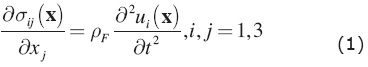
Where: ρ_F=density of the fluid. If we consider that stresses in the fluid are related to the pressure generated by the incident pulse, subsequently, one can express this last equation as:

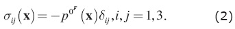
Therefore, the displacement field in the fluid can be represented by its well-known form:

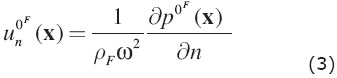
The incident pulse at the fluid, as shown in Fig. 1a (inset), can be given as:

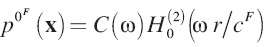
where p^oF(X)=incident pulse at the fluid, x = {x₁,x₃} ,c(ω)=scale factor for the incident pulse, H₀⁽²⁾(•) =Hankel function of second kind and zero order, ω=circular frequency, c^F=compressional wave velocity in the fluid and r=r(x) is the distance from the receiver to the source.

Integral representation for diffracted wave fields

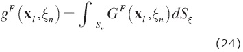
To represent the diffracted wave fields (for pressures and displacements) in the fluid due to the incident pulse impacting the solid medium (elastic solid wall), we suggest the following integral representations:

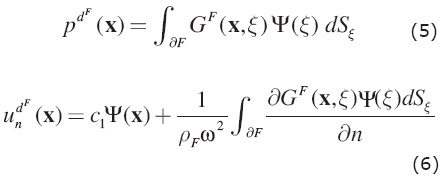
where,

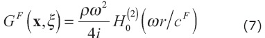
ψ(•)=force density for the fluid, G^F (•) = Green function for the fluid, and c₁ defines the region orientation and can assume a value of -0.5, 0 or 0.5 (see explanation for c₂, given below).

The whole pressure and displacement fields in the fluid, besides, free and diffracted one, can be expressed, respectively, by:

Since the source is only applied to the fluid, it is expected that, in the solid, only diffracted waves will appear and they can be established as follows.

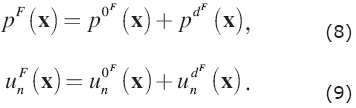
Consider a domain V, bounded by the surface S. If this domain is occupied by an elastic material, the displacement field under harmonic excitation can be written, neglecting body forces, by means of the single-layer boundary integral equation as follows:

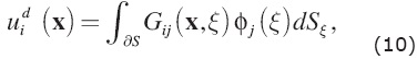
where u_i(x)= i -th component of the displacement at point x, Gij(x;ξ) = Green's function, which is the displacement produced in the direction i at x due to the application of a unit force in direction j at point ξ, Φ is the force density in direction j at point ξ (the subscripts i, j are restricted to be 1 or 3 and the summation convention is applied, i.e. a repeated subscript implies summation over its range, 1 and 3 in this case). This integral representation can be obtained from Somigliana's identity (Sanchez-Sesma, 1991).

This integral representation allows the calculation of stresses and tractions by means of the direct application of Hooke's law and Cauchy's equation, respectively, except at boundary singularities, that is, when x is equal to ξ on surface S. From a limiting process based on equilibrium considerations around an internal neighborhood of the boundary, it is possible to write, for x on S,

where t_i(x) is the i-th component of traction, c₂=0.5 if x tends to the boundary S "from inside" the region, c₂=-0.5 if x tends S "from outside" the region, or c₂=0 if x is not at S. T_ij(x;_i) is the traction Green's function, that is to say, the traction in the direction i at a point x, associated to the unit vector n_i(x), due to the application of a unit force in the direction j at ξ on S. The two-dimensional Green's functions for an unbounded space can be found in (Rodrfguez-Castellanos et al., 2007; and Avila-Carrera et al., 2009).

Boundary Cond/t/ons

In the IBEM is convenient to divide the domain into two regions (S for the solid and F for the fluid), in which proper boundary conditions that represent the problem under consideration have to be established. These boundary conditions for fluid-solid interfaces can be expressed as:

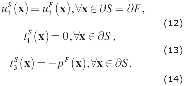
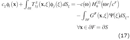
Writing the boundary condition (12) as function of the diffracted field (10) for the solid and incident (3) and diffracted (6) fields for the fluid, we obtain:

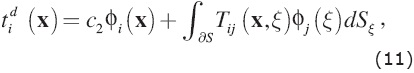
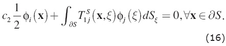
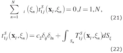
The condition traction free (13) can be expressed from the integral form (11), obtaining,

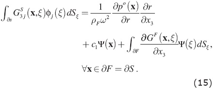
The boundary condition (14), can be written by means of (11), (4) and (5), and then we have

Discretization scheme

In this section, we show the discretization of the Eqs. (15) to (17). Assuming that force densities Φ(x) and ψ(x) should be constant on each element that forms the surfaces of regions S and F, respectively, and Gaussian integration (or analytical integration, where the Green's function is singular) is performed, then, Eq. (15) can be written as,

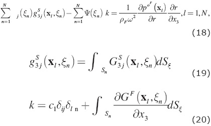
Eq. (16) leads to:

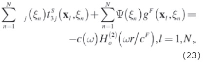
Eq. (17) can be expressed as:

Eqs. (18), (21) and (23) form a system of integral equations that has to be solved and, therefore, force densities Φ(x) and ψ(x) can be found. Once the force densities have been obtained, the whole displacement and pressure fields in the fluid can be found by means of Eqs. (8) and (9). For the solid, the entire traction and displacement fields can be obtained by means of Eqs. (10) and (11).

 

Brief description of the formulation by means of the discrete wave number

The discrete wavenumber method is one of the techniques to simulate earthquake ground motions. The seismic wave radiated from a source is expressed as a wavenumber integration (Bouchon and Aki, 1977). The main idea of the method is to represent a source as a superposition of homogenous plane waves propagating in discrete angles. As long as the medium has no inelastic damping, the denominator of the integrand becomes zero for a particular wavenum-ber and, consequently, the numerical integration becomes impossible. To solve this problem, a method to incorporate a complex frequency was proposed as early as the proposal of the discrete wavenumber method itself (Bouchon and Aki, 1977).

The incident pulse in the fluid, as shown in Fig. 1a (inset), can be given as:

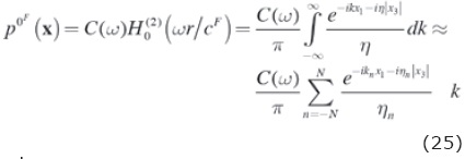
where,

k=the wavenumber, with Im η< 0. If we express k in discrete values then we have k_n=n k and η_n= 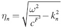with Im η_n< 0.

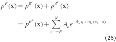
If we assume that the whole pressure field in the fluid is represented as the sum of free field and diffracted one, then, it can be expressed, respectively, by:

and

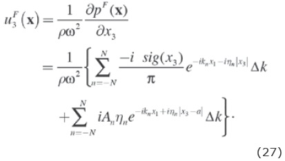
For the solid, we assume that potential of displacement has the form and , with Im γ_n<0. αand βare the compressional and shear wave velocities, respectively.

The displacement field for the solid can be expressed as and .

The stress field is obtained by the well-known equation:

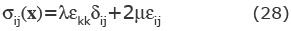
where σ_ij(x)=stress tensor, λ and μ are the Lame's constants, ε_ij=strain tensor and δ_ij Kronecker's delta.

The boundary conditions to be applied are represented by Eqs. (12) to (14). Once the boundary conditions have been applied, the unknown coefficients A_n, B_n and C_n are obtained and the whole pressure field in the fluid is finally determined by means of the Eq. (26).

 

Testing and numerical examples

To test the accuracy of our formulation, we selected several interface cases considering a broad range of properties (soft to hard) of solid materials, characterized by their wave propagation velocities and densities. The material properties that were used in the calculations are shown in Table 1, where six cases are presented.

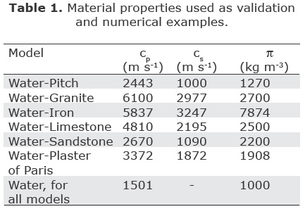
Compressional wave velocity, c_p, shear wave velocity, c_s, and mass density, π, were included in Table 1. These materials were previously considered by Borejko (Borejko, 2006), who developed theoretical and experimental techniques to show the emergence of interface waves in several materials like those from Table 1. His results showed good agreement between theoretical and experimental results.

Figure 1 shows the pressure spectra for the six models analyzed for which the wave propagation velocities and densities are displayed in Table 1. For all cases, the initial pressure (source) was generated at a distance of 0.05 m (see inset in Fig.1a) from the elastic solid boundary. The receiver is placed at a horizontal distance of 1.0 m from the source (as shown in the detail of Fig. 1a). The frequency analysis is done considering a frequency increment of 150 Hz and reaching a maximum of 19200 Hz. The discretized surface is located between x₁=-3.5 m and x₁=3.5 m, within this interval spurious waves inside the zone of interest were eliminated. Moreover, 6 boundary elements per S-wave wavelength were considered.

In this figure, the results obtained by the IBEM (dotted line) and by DWN (continuous line) are displayed. There is an excellent agreement between the two methods for the frequency range studied. It can also be seen that for the models of Water-Pitch and Water-Sandstone, resonant effects are slightly manifested. However, in both cases, from the frequency of 6000 Hz, the curves describe a performance almost identical and become asymptotic. This behavior can be attributed due to the fact that their shear wave velocities are lesser than the compressional wave velocity for the fluid.

For all other models (Figures 1b, c, d, f) the spectrum of pressure shows a simple and monotonous behavior, describing oscillations of small-scale in every case. One can notice that for the Figure 1a and e the pressures registered are almost negligible, after 6000 Hz.

Figures 2a and b show the time response for the complete 2D Water-Pitch interface model. For this analysis, a grid of 51 x 51 receivers, spaced using a distance increment of 0.04 m, is used. Column a) shows the results of pressure in the fluid and displacements in the x₁ direction for the solid, while, column b) shows pressures in the fluid and displacements in the x₃ direction for the solid. This phenomenon is shown for three different times.

For the time t=0.000911 s, the initial wave of pressure has hit the solid boundary and a reflected wave in the fluid and diffracted waves in the solid can be seen, generating the emergence of P and S wave fronts. For the time t=0.001432 s, the above mentioned waves go away from the source while the presence of interface waves is clearly evident to this instant. These are the Scholte's waves and are highlighted using circles in Figures 2a and b. For the time t=0.001953 s, the propagation of interface waves is very visible and shows a delay with respect to the P and S wave fronts in the solid. Scholte's waves for this case propagates with a velocity of 823.5m s^-1.

Figures 2c includes synthetic seismograms of pressures (top figure), x₁ horizontal displacement (middle figure) and x₃ vertical displacement (bottom figure) for seven receivers located near to the interface. The first receiver is located at a horizontal distance of 0.50 m from the source and the others are separated every 0.25 m.

In the seismogram of pressures, the last wave front corresponds to the Scholte's waves, which clearly carry the most of interface energy, as expected. The same effect can be seen in the case of displacement seismograms. It is relevant to note that for the x₃ direction displacement amplitudes are larger than those for the x₁ direction. This can also be seen in Figures 2a and b (middle and bottom).

Figure 3 displays results in time domain for the materials shown in Table 1. The material tagged with " * " was added for comparison with regard to the results published by Strick and Ginzbarg, and Strick et al. (Strick and Ginzbarg, 1956; Strick et al, 1956). The properties for this material (Sandstone* in Fig. 3) are c_p=3740 m s^-1, c_s=1645 m s^-1 and density of 2400 kg m^-3. The location of the receiver is illustrated in Figure 1a, for all the cases. Synthetic seismograms in this figure were placed considering the shear wave velocity of each material. The highest speed corresponds to Steel (c_s= 3247 m s^-1) and the lowest to Pitch (c_s= 1000 m s^-1). The time is normalized with regard to the compressional wave velocity c_p=1501 m s^-1 (velocity of water) and r₁, which is the distance from the image source and the receiver. In this figure, pressures registered by the receiver (for each material) are plotted.

The pressure waves diffracted by rigid interfaces (as Granite and Steel) show higher values, while, those diffracted by less rigid interfaces, like Sandstone and Pitch, show lower values. Additionally, for these last two cases, the wave fronts tend to be less noticeable. Arrivals of P and Scholte's wave fronts are indicated using dashed-dot lines.

For comparative purposes, Scholte's wave front obtained by Strick and Ginzbarg, and Strick et al. (1956) is also included. This is represented with stars in the figure, good agreement between the results is observed. It is clear that the Scholte's wave is evident from the Limestone and manifests a significant delay for the Pitch.

Finally, a sinusoidal interface is considered. Figure 4a shows the model used to deal with this geometry. Material properties for this case are: for the elastic medium c_p=3400 ms¹, c_s=1963 ms^-1 and p=2500 ms^-1, while for the acoustic one c_p=1500 ms^-1 and p=1020 kgm^-3. The source time function is a Ricker wavelet with a dominant frequency of 10 Hz. The source and receiver locations are depicted in Figure 4a. Synthetic seismograms are shown in Figure 4b and c for vertical and horizontal displacements, respectively. Results by IBEM are plotted with a dotted line, while those obtained by means of the Spectral Element Method (SEM, Komatitsch et al. 2000), are drawn with a solid line. The agreement between both methods is good. Here, the direct wave is clearly observed since the source point and the receiver are very close to each other. Moreover, multiple reflections are presented because of the interactions between the direct wave and the sinusoidal interface, as expected; this effect is clearly seen in Figure 4b and c. The possibility of modeling arbitrary interface shapes is one of the main advantages of the IBEM. Additionally, another advantage of this method relies on the use of Green's functions for unbounded space, which have a simple form and can be easily programmed. The use of these functions has provided accurate numerical results.

 

Conclusions

In this paper we extended the use of the Indirect Boundary Element Method to study the propagation of elastic waves in fluid-solid interfaces. In this numerical technique, based on the Huygens' principle and the Somigliana's representation theorem, the fields of pressures and displacements are expressed in terms of single layer boundary integral equations. Full space Green's functions for tractions and displacements are used, but they are forced to meet the proper boundary conditions that prevail at the fluid-solid interfaces.

A wide range of solid materials characterized by their wave velocities and densities was analyzed. In every case, the presence and propagation of Scholte's waves is noticed, highlighting the important amount of energy that they carry.

The results obtained from our numerical technique were compared with those obtained by the DWN and SEM. Therefore, we conclude that there is a good agreement between the different approaches studied.

 

References

António J., Tadeu A., Godinho L., 2005, 2.5D scattering of waves by rigid inclusions buried under a fluid channel via BEM, European Journal of Mechanics A/Solids 24, 957-973.         [ Links ]

Avila-Carrera R., Rodríguez-Castellanos A., Sánchez-Sesma F.J., Ortiz-Aleman C., 2009, Rayleigh-wave scattering by shallow cracks using the indirect boundary element method. J. Geophys. Eng. 6, 221-230.         [ Links ]

Biot M.A., 1952, The interaction of Rayleigh and Stoneley waves in the ocean bottom. Bull. Seism. Soc. Am. 42, 81-93.         [ Links ]

Borejko P., 2006, A new benchmark solution for the problem of water-covered geophysical bottom. International Symposium on Mechanical Waves in Solids, Zhejiang University, Hangzhou, China, 15-16 may 2006.         [ Links ]

Bouchon M., Aki K., 1977, Discrete wave number representation of seismic source wave fields. Bull. Seismol. Soc. Am. 67, 259-277.         [ Links ]

Carcione J.M., Helle H.B., 2004, The physics and simulation of wave propagation at the ocean bottom. Geophysics 69, 825-839.         [ Links ]

Carcione J.M., Helle H.B., Seriani G., Plasencia-Linares M.P., 2005, Simulation of seismograms in a 2-D viscoelastic Earth by pseudospectral methods. Geofisica Internacional 44, 123-142.         [ Links ]

Eriksson A.S., Bostrom A., Datta S.K., 1995, Ultrasonic wave propagation through a cracked solid. Wave Motion 22, 297-310.         [ Links ]

Ewing W.M., Jardetzky W.S., Press F., 1957, Elastic waves in layered earth, McGraw-Hill Book Co.         [ Links ]

Godinho, L., Tadeu, A., Branco, F., 2001, 3D acoustic scattering from an irregular fluid waveguide via the BEM. Engineering Analysis with Boundary Elements J. 25, 443-453.         [ Links ]

Gurevich B., Ciz R., 2006, Shear wave dispersion and attenuation in periodic systems of alternating solid and viscous fluid layers. International Journal of Solids and Structures 43, 7673-7683.         [ Links ]

Komatitsch D., Barnes C., Tromp J., 2000, Wave propagation near a fluid-solid interface: a spectral-element approach. Geophysics 65, 623-631.         [ Links ]

Mayes M.J., Nagy P.B., Adler L., Bonner B., Streit R., 1986, Excitation of surface waves of different modes at fluid-porous solid interface. J. Acoust. Soc. Am. 79, 249-252.         [ Links ]

Meegan G.D., Hamilton M.F., Yu. Il'inskii A., Zabolotskaya E.A., 1999, Nonlinear Stoneley and Scholte waves. J. Acoust. Soc. Am. 106, 1712-1723.         [ Links ]

Nayfeh A.H., Taylor T.W., Chimenti D.E., 1988, Theoretical wave propagation in multilayered orthotropic media. Applied Mechanics Division), Wave Propagation in Structural Composites 90, 17-27.         [ Links ]

Rayleigh J.W.S., 1885, On waves propagated along the plane surface of an elastic solid. Proc. London Math. Soc. 17, 4-11.         [ Links ]

Rodríguez-Castellanos A., Ávila-Carrera R., Sánchez-Sesma F.J., 2007, Scattering of Rayleigh-waves by surface-breaking cracks: an integral formulation. Geofisica Internacional 46, 241-248.         [ Links ]

Rodríguez-Castellanos A., Flores-Mendez E., Sánchez-Sesma F.J., Rodriguez-Sanchez J.E., 2010, Numerical formulation to study fluid-solid interfaces excited by elastic waves. Key Engineering Materials 449, 54-61.         [ Links ]

Sanchez-Sesma F.J., Campillo M., 1991, Diffraction of P, SV and Rayleigh waves by topographic features; a boundary integral formulation. Bull. Seism. Soc. Am. 81, 1-20.         [ Links ]

Scholte J.G., 1942, On the Stoneley wave equation. Proc. K. Ned. Akad. Wet. 45 Pt. 1: 20-25, Pt. 2: 159-164.         [ Links ]

Scholte J.G., 1947, The range of existence of Rayleigh and Stoneley waves. Mon. Not. R. Astron. Soc. Geophys. Suppl. 5, 120-126.         [ Links ]

Stoneley R., 1924, Elastic waves at the surface of separation between two solids. Proc. R. Soc. London, Ser. A 106, 416-428.         [ Links ]

Strick E., Ginzbarg A.S., 1956, Stoneley-wave velocities for a fluid-solid interface. 46, 281-292.         [ Links ]

Strick E., Roever W.L., Vining T.F., 1956, Theoretical and Experimental Investigation of a Pseudo-Rayleigh Wave. J. Acoust. Soc. Am. 28, 794.         [ Links ]

Thomas C., Igel H., Weber M., Scherbaum F., 2000, Acoustic simulation of P-wave propagation in a heterogeneous spherical earth: numerical method and application to precursor waves to PKP. Geophys. J. Int. 141, 6441-6464.         [ Links ]

Van Vossen R., Robertsson J.O.A., Chapman C.H., 2002, Finite-difference modeling of wave propagation in a fluid-solid configuration. Geophysics 67, 618-624.         [ Links ]

Wang J., Zhang C., Jin F., 2004, Analytical solutions for dynamic pressures of coupling fluid-solid-porous medium due to P wave incidence. Earthquake Engineering and Engineering Vibration 3, 263-271.         [ Links ]

Yoshida M., 1978a, Velocity and response of higher mode Rayleigh waves for the Pacific Ocean. Bull. Earthq. Res. Inst. 53, 319-338.         [ Links ]

Yoshida M., 1978b, Group velocity distributions of Rayleigh waves and two upper mantle models in the Pacific Ocean. Bull. Earthq. Res. Inst. 53, 1135-1150.         [ Links ]

Zienkiewicz O.C., Bettess P., 1978, Fluid-structure dynamic interaction and wave forces, an introduction to numerical treatment. J. Numer. Meth. Eng. 13, 1-16.         [ Links ]