Article

 

A test of the effect of boundary conditions on the use of tracers in reservoir characterization

 

M. Coronado¹*, J. Ramírez–Sabag¹, O. Valdiviezo–Mijangos¹ and C. Somaruga²

 

¹ Instituto Mexicano del Petróleo, México City, Eje Central Lázaro Cárdenas 152, Deleg. G. A. Madero, 07730, City, México. ^*Corresponding author: mcoronad@imp.mx

² Facultad de Ingeniería, Universidad Nacional del Comahue, Neuquén, Buenos Aires 1400, 8300, Argentina.

 

Received: March 27, 2007
Accepted: November 5, 2008

 

Resumen

El establecimiento de condiciones de frontera adecuadas en modelos de transporte de trazador ha sido un tema controvertido principalmente debido a insuficiente evidencia física. En nuestro trabajo se analiza el problema desde una perspectiva orientada a la práctica. Se ajustan dos modelos equivalentes, pero con condiciones de frontera distintas, a una misma serie de datos de una prueba de trazadores y los valores resultantes de los parámetros de ajuste se comparan entre sí. La relevancia de las condiciones de frontera será alta si los valores difieren importantemente. El sistema considerado es la inyección de un pulso de trazador en un medio homogéneo unidimensional, en el cual el pulso se mueve a velocidad constante sujeto a advección y dispersión. El primer modelo establece condiciones sobre la concentración de trazador y el segundo sobre su flujo. Se encontró que las condiciones de frontera se vuelven más relevantes a menores números de Peclet. En los casos analizados el número Peclet es 25.0, 5.4 y 3.7 respectivamente; ello dio lugar a una diferencia máxima en el valor de los parámetros de ajuste de 5%, 18% y 37%. Aunque grande para experimentos de laboratorio, este porcentaje es en general poco significativo en pruebas de trazadores en campos petroleros, pues la variabilidad en los datos es frecuentemente alta. El uso de ciertas condiciones de frontera en lugar de otras parece no tener consecuencias importantes en la caracterización de yacimientos petroleros, sin embargo se debe tener cuidado cuando se tengan números de Peclet pequeños.

Palabras clave: Trazador, soluto, condiciones de frontera, transporte, yacimiento petrolero, problema inverso.

 

Abstract

Tracer tests are fundamental in characterizing fluid flow in underground formations. However, the setting of appropriate boundary conditions in even simple analytical models has historically been controversial, mainly due to the lack of sufficient physical evidence. Determining the relevance of boundary conditions on tracer test analysis becomes therefore a topic of renewed interest. The subject has been previously disscused by studying the tracer breakthrough curve sensitivity to diverse model parameter values. In our present work we examine the issue from a new practical reservoir characterization perspective. Two well–known equivalent elementary tracer transport models having different boundary conditions are matched to the same tracer test data. The resulting model parameter difference quantifies the effect of boundary conditions on reservoir property determination. In our case a tracer pulse injected in a homogeneous one–dimensional porous medium and moving at constant speed dominated by advection and dispersion is considered. The tracer transport models to be used yield conditions (i) on the tracer concentration, and (ii) on the tracer flux. Three data sets from tracer tests performed in different oil reservoirs are used to fit the models and determine the parameter values. We found that boundary conditions become more important as Peclet number gets smaller. The cases analyzed have Peclet numbers 25.0, 5.4 and 3.7. The largest parameter difference obtained in each case is 5%, 18% and 37% respectively. These differences are large for laboratory experiments, but less relevant for tracer tests in oil fields, where data variability is frequently high. Nevertheless, attention should be paid when small Peclet numbers are present.

Key words: Tracer, solute, boundary conditions, transport, oil reservoir, inverse problem.

 

Introduction

Analytical and numerical tracer transport models are regularly employed in the design and interpretation of field tracer tests. Particularly, the estimation of porous formation properties is searched by fitting models to real data. Along the years multiple analytical models has been developed, however the selection of appropriate boundary conditions has been the subject of many discussions, mainly since actual flow border conditions are in reality not well known (Gershon and Nir, 1969; Kreft and Zuber, 1978; Parker and van Genuchten, 1984; Kreft and Zuber, 1986; Novakowski, 1992; Schwartz et al. 1999; Coronado et al, 2004). For practitioners, the selection of an appropriate model to describe a given field tracer test becomes a hard issue, since multiple border conditions are available, model properties and limitations are in many cases not clearly described in the literature. A relevant practical and simple work in this context is therefore the quantification of the consequences that might appear by choosing certain boundary condition over other conditions. This issue has been partially studied previously by analyzing the sensitivity of tracer breakthrough curves to the diverse model parameters. Through these calculations the importance of the Peclet number has become apparent (Gershon and Nir, 1969; van Genuchten and Alves, 1982). In this work we examine the problem from a practical perspective. We quantify the border condition impact on the reservoir characterization by fitting equivalent models having different boundary conditions to the same tracer breakthrough data set. From diverse models different parameter values can appear. If only a small value difference results, it would then mean that the border condition issue is not significant. Different boundary conditions would then yield in this case similar results regarding porous media characterization.

To examine the proposed approach, we consider in this paper the basic and simple situation of the advective–dispersive transport of a tracer pulse in semi–infinite homogeneous one–dimensional porous medium moving at uniform fluid velocity. Diverse models are available in the literature for this case (see for example Bear, 1972; Kreft and Zuber, 1978; van Genuchten and Alves, 1982). Two of these models are chosen for our calculations, a traditional model that sets the pulse condition on the tracer concentration, and a different model, that gives the pulse condition on the tracer flux. The second model has sounder physical grounds and corresponds to the so called flux concentration condition (Kreft and Zuber, 1978), while the first one applies strictly only when dispersion effects are negligible (piston like behavior). Both models are to be matched to the same data sets obtained from three different field tracer tests. The models are very briefly described in the next section. In the next section the optimization approach is presented. The model fitting using data from tracer tests performed in the Ranger Field, Loma Alta Sur Field and Carmopolis Field is shown in a subsequent section. Conclusions are drawn in the final section.

 

The models

The system under consideration corresponds to an underground channel connecting an injection well to a distant production well in a reservoir, as displayed in Fig.1. In order to apply the simple models previously mentioned an important simplification should be made: we assume a uniform communication channel having a constant volumetric fluid flow rate Q, a constant cross–section S, and a flow effective porosity . Here, the corresponding interstitial uniform fluid velocity is given by u =Q / S . The actual flow pattern near a well is radially divergent or convergent, however in diverse multi–well situations this pattern type is just a local feature, not a global characteristic. The constant velocity assumption is quite restrictive, but it can roughly apply in cases with longitudinally large and laterally limited underground structures that are locally homogeneous. This can be the situation in underground formations of fluvial origin, when the injection and the production wells are both localized within the same rubber–shape structure. The tracer transport in this one–dimensional semi–infinite system will be also assumed to be fully dominated by advection and dispersion. The tracer dispersion coefficient, D, is taken constant and linearly proportional to the velocity, as empirical results might suggest. Hence, the tracer mass conservation equation becomes ∂ C/∂ t + u∂ C/∂ c – D∂ ²C /∂ x², where C(x,t) is tracer concentration.

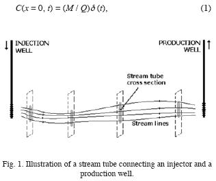
The traditional model for tracer pulse injection to be used here gives conditions on the tracer concentration at the injection border, x = 0, as

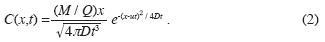
being δ(t) a Dirac delta function in time, and M the total mass introduced in the system (here the communication channel). This condition imposes in reality a non–physically feasible tracer concentration pulse at the border if dispersion is present. The solution obtained by setting the downstream condition C(x ∞, t) = 0 is (Lenda and Zuber, 1970)

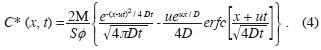
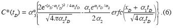
In this paper we compare the model from Eq.(2) against a model that introduced the pulse not on the concentration but on the tracer flow, J =uC – D∂ C/∂ x, as

The solutions is (Kreft and Zuber, 1978)

Equations (2) and (4) implicitly involve a fundamental parameter commonly appearing in tracer transport models, which is the Peclet number, Pe = uL / D, with L the distance between the injection and the observation site. This number is a key parameter in determining the relevance of boundary conditions. By studying tracer breakthrough curve sensitivity to the Peclet number in the case of continuum tracer injection, Gershon and Nir (1969) found that diverse boundary conditions yield tracer breakthrough differences which reduce by increasing the Peclet number. For Pe=100 they observed a difference of 5%. Also for continuous tracer injection, Van Genuchten and Alves (1982) compared semi–infinite and infinite x–domain models with boundary conditions given as the tracer concentrations and as the tracer flow. They found that tracer breakthrough curves get similar by increasing the Peclet number form 5 to 60. For a semi–infinite system the largest concentration value difference found at Pe = 5 is 15%. For Pe = 20 this difference reduce to 7%. They comment that differences are roughly of the same order of magnitude as experimental error, and that effects of the boundary conditions analyzed can be neglected for Pe > 20. In finite–step injection similar results have been found, where breakthrough curve differences decrease in around 40% when changing the Peclet number from 5 to 20 (Coronado and Ramírez–Sabag, 2005).

We can directly compare the tracer breakthrough curve obtained from the model in Eq.(2) to the curve from the model in Eq.(4) for diverse Pe – values by calculating at x = L the time integral of the curve C(t) – C* (t) and dividing it by the time integral of the curve C* (t). As known previously, differences increase by reducing the Peclet number. For Pe = 10 the relative curve difference is approximately 19%. This value increases to about 27% for P_e = 5 and reduces to 13% for P_e = 20. To determine the actual impact of the border conditions on reservoir characterization, the two models will be fitted to various field tracer test data sets. In this case, an inverse problem is to be solved, which is subject of the next section.

 

The optimization procedure

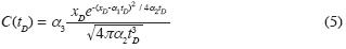
In order to match the analytical models presented in Eqs. (2) and (4) to field tracer breakthrough data, it is convenient to change variables and parameter into a more adequate dimensionless form. The space and time variables x and t are transformed to variables that does not involve any of the three fitting parameters D, u and M. We therefore choose x_D = x / L and t_D = t / t_R, where L is a representative interwell distance, and t_R is a representative tracer transit time obtained from the tracer data. The final results will not depend on the L and t_R chosen. The new model parameters are defined as α₁ = ut_R / L, α₂ = Dt_R / L², α₃ = M / uSt_R and α₃* = M / LS. The so called scale parameter is α₃ for the model in Eq. (2) and α₃ * for the model in Eq. (4). The α₃ s are linked with each other by α₃* = α₃α₁ . Parameters and α₁ are α₂ dimensionless, while α₃ and α₃* have dimensions of concentration. By introducing the new quantities in Eq. (2) and Eq. (4) it follows

and

After data fitting the effective velocity and dispersion coefficient can be recovered from α₁ and α₂ as u = α₁ L/t_R and D = α₂L²/t_R .The Peclet number is given by Pe = α₁/ α₂. From α₃ or α₃* the value M/S can be obtained, and introducing the total tracer amount recovered, the interstitial effective sweep channel cross–section, S, can be evaluated. This cross–section is commonly not computed in tracer test interpretations. Models are regularly fitted to previously normalized data, loosing therefore reservoir information involved in the scale parameter.

A critical issue when applying regression methods is the identification of a global minimum over the multiple local minima that might be present. Various approaches can be followed to reduce uncertainty on the global minimum. In this work we take the procedure described by Ramírez–Sabag et al. (2005). This scheme is based on the fact that different optimization methods follow different search paths; thus by applying various selected regression methods to the same problem a broad view of the solution set is obtained. When combining this scheme with a parameter sensitivity analysis the selection of the global minimum is commonly highly reliable. In a sensitivity analysis the variation of the objective function with respect to the fitting parameters is examined, thus global and local minima can be observed (Dai and Samper, 2004). The objective function to be minimized in this paper is a sum of non–weighted squared differences. In this work the standard optimization methods Nelder–Mead, Gauss–Newton, Levenberg–Marquardt and Steepest–Descent were employed (Ramírez–Sabag et al., 2005). The starting parameter values chosen for regressions were α₁ = 1 and α₂= 0.1. No starting value is required for a₃ since it is a linear multiplicative parameter. The fixed value x_D = 1 was established, i.e. the observation point is located at the production well distance, i.e. x = L. Accordingly to the system characteristics, the parameter ranges analyzed were α₁ [0.2, 5]and α₂[0.02, 0.5].

 

Field tracer test cases

Multiple tracer tests have been performed in oil reservoirs to investigate flow performance and reservoir properties that control water or gas displacement proces ses, as well as to determine residual oil saturation (Du and Guan, 2005). Tracer breakthrough data from various tests are published in the literature, some of them can be used in this work, provided certain conditions hold. Among other issues it should be examined: reservoir structure, test conditions, tracer type, wells involved and tracer data structure. Some desirable tracer test requirements to apply the one–dimensional models described above are that reservoir formation should not be fractured, and should have stripe–like or lens structures where uniform flow can develop, as in fluvial origin reservoirs. Water production should be high, thus main flowing fluid is water, and oil saturation should be low, preferable close to the irreducible oil saturation (non–mobile oil). Injection and production rates should be constant in order to have steady–state. Tracer should be non–particionable, with negligible adsorption and be injected as a pulse. Moreover, we preferentially take smooth bell–shaped breakthrough data sets with a single peak and low data dispersion, which might indicate that just a single communication channel is involved. . In general not all these requirements are simultaneously fulfill in the data cases available, nonetheless we have found three good prospects. They correspond to tracer tests performed in the oil reservoirs Ranger Field in Texas, Loma Alta Sur Field in Argentina, and Carmopolis Field in Brazil.

We emphasize that the main objective of our model matching is a simple comparison between the properties obtained by using Eq. (5) versus Eq. (6), not a detailed description of the tracer test and reservoir characterization.

The Ranger field

Diverse tracer tests were performed in the McClesky Sandstone of the Ranger Field in Texas in order to characterize reservoir communications in relation to a surfactant–polymer flood aiming improved hydrocarbon recovery (Lichtenberger, 1991; Allison et al. 1991). To this purpose, various tracers in different injection wells before and after the polymer flood were introduced, and the changes in the communication pattern observed. In this work we analyze the specific tracer data of a 10 Ci tritiated water pulse injection in Well 38 and its arrival in Well 40, which is 281 m apart. This well pair was selected since a high permeability communication channel seems to be present in the most relevant formation layer of this region. Further, as reported by Allison et al (1991) for this area, the average oil saturation was estimated in 0.39, which is a value similar to the global irreducible oil saturation of 0.38 estimated by core studies. Hence, the main moving reservoir fluid is water, what is consistent with the low oil production in Well 40. From the diverse tracer data available we have chosen tritiated water data, since it is a non–particionable tracer (although indications of low Tritium exchange with immobile Hydrogen appear), and since the breakthrough curve main peak shows the presence of just a single communication channel. Additionally, we took these wells since the streamline pattern (Lichtenberger, 1991) suggests a relatively uniform flow pattern.

As previously mentioned, our main interest in this work is the comparison of the fitting, the detailed conclusions regarding the polymer flood efficiency are outside the scope of this manuscript. Tracer concentration data in this test are given in percentage (of the tracer amount inject) per liter. As a reference time we select the mean transit time, which is t_R = 250 days, by this way t_d takes values that are close to unity.

The data fitting procedure yields a single solution for both models in Eqs. (5) and (6). It has been verified by parameter sensitivity plots, such as those illustratively shown in Fig. 2 for the case of Eq. (5). In these plots the objective function in terms of one of the parameters α₁ α₂ and α₃ is displayed, while keeping the other two parameters fixed. The fixed parameter values employed in this figure were α₁ = 1.0, α₂ = 0.1 and α₃ = 4.0. Other sensitivity plots, as those in Fig. 2, show a single global minimum in the relevant parameter range. Similar plots appear for the case of the model in Eq. (6). Thus, the uniqueness of the solutions is guaranteed. Indeed, diverse optimization methods yield the same solution.

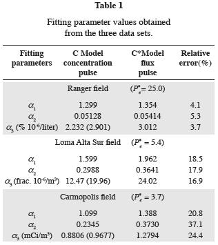
The final regression curves are shown in Fig. 3. The original tracer data are displayed as circles, the fitting curve for model C as a broken line, and the curve for model C* as a solid line. Data matching is good. The solid line coincides with the broken line exactly. Thus, the optimization gives fully similar curves, but different model parameter values. Table 1 lists the fitting parameters obtained from the optimization procedure. It can be seen that the relative parameter difference is near 5% for α₁ and α₂. The α₃ –value is 2.23, which for comparison purposes should be transformed as α₃ → α₃α₁ = 2.901 (value shown in parenthesis in Table 1). This value should be faced up against α₃* = 3.012. The difference in the parameter α₃ is close to 4%. We conclude that discrepancies on all fitting parameters are less than or around 5%. The corresponding Peclet number for this tracer test is Pe* = α₁* / α₂* = 25.0.

The Loma Alta Sur field

Loma Alta Sur is a highly heterogeneous fluvial oil reservoir having long sandstone bodies with reduced lateral continuity. The field is on a mature stage and diverse enhanced oil recovery projects have been studied. Various tracer tests were performed to determine reservoir hydraulic connectivity (Badessich et al. 2005). The tracer data set employed in this paper corresponds to tritiated water injection in well LAS–56 and its arrival at well LAS–47. The field average water saturation is 70% and the oil production in LAS–47 is less than 5%, thus main flowing fluid is water. As a reference transit time we take the peak concentration time, which is t_R = 30 days. The inter–well distance is L = 133 m; it is approximately half the well distance of the previous field case. As in that case, a single global minimum solution appears from the optimization methods. The fitting parameters obtained are listed in Table 1, and a plot of the fitting curves is shown in Fig. 4. Data matching is satisfactory. Here, some small differences between the C and C* curves can be appreciated. The parameter discrepancy is about 18% for a₁ and a₂ The α₃ value is 12.47, which transforms as α₃ → α₃ α₁ = 19.96 to be compared with α₃* = 24.02. It leaves a 17% error. We conclude that the general parameter error is near 18% in this tracer test, which is close to four times larger than in the Ranger Field case. The Peclet number is P_e* = 5.4, which is four times smaller than the previous case.

The Carmopolis field

The Carmopolis field is a sandstone and conglomerate mature reservoir with two main layers. Here, diverse improved oil recovery schemes have been considered. The average water saturation is 50%, and the global water to oil production ratio is 5. In analyzing a polymer injection project for mobility control various tracer tests were performed in a non–fractured pilot area subject to water injection. In particular, two tracers were injected in well I–1: tritiated water was introduced before the polymer injection and fluorescein after it (de Melo et al., 2001). Tracer arrivals were monitored in the four surrounding production wells. The specific tracer breakthrough examined in this paper is the injection of 996 mCi tritiated water and its arrival at the production well P–4 located at 63 m from it. This distance is near half the distance of the Loma Alta Sur case and a fourth of the Ranger Field situation. Tritiated water is a conservative tracer. Laboratory tests indicate a low Tritium rock absorption of 2.6%. The tracer breakthrough data selected show a single smooth peak, which corresponds to the flow in one production layer. Data are given in terms of the cumulative reservoir fluid production, V = q t, where q and t are the fluid production rate and the time, respectively. We therefore make the analysis in terms of cumulative production instead of the time. Equations (5) and (6) maintain their form, but with a dimensionless cumulative production V_d = V / V_R instead of t_d . V_R is a reference cumulative production, which was taken here as the transit average, which is 150 m³. As mentioned before, this selection has no effect on the final results, it is just to define an adequate dimensionless cumulative production, V_d . The new fitting parameters are α₁ = uV_R / qL, α₂ = DV_R / qL² and α₃ = (M /S)(q/uV_R) or α₃ = M /SL = α₃ α₁ . In Fig. 5 the fitting curves and the original field data are displayed. The resulting optimized parameter values are shown in Table 1. Again, a single global solution was found. The parameter differences found in α₁ and α₂ are larger than in the Loma Alta Sur, here they are 21% for α₁ and 37% for α₂. The effective α₃ discrepancy is 24%. In this tracer test Pe* = 3.7 was obtained.

 

Summary and concluding remarks

There have been many paper published in the literature on boundary conditions to be used in describing tracer transport in underground formations, however the subject is presently still not conclusive. The selection of a model having appropriate boundary conditions to describe a given tracer test can become ambiguous, specifically for practitioners, since model limitations are frequently not discussed in the literature, and even further, some traditional border conditions have been described as physically improper. An important application of tracer tests is the characterization of a porous formation. To this purpose tracer test data are fitted to tracer transport models and the resulting parameters used to evaluate formation properties. Thus, a model with certain boundary conditions can yield parameter values that are different from an equivalent model with other boundary conditions. The question is, how different the obtained reservoir properties would get if certain boundary conditions were employed instead of the original conditions used. In this work we approach to an answer by considering a well–known simple one–dimensional advection–dispersion tracer pulse transport model, and comparing the parameter values resulting from a boundary condition established in the tracer concentrations against a condition established on the tracer flux. Data from three published field tracer tests are used to fit the two models under consideration. To perform the data fitting an inverse problem is solved by a technique that makes use of various optimization methods and a parameter sensitivity analysis. The tracer data employed are from the Ranger Field in Texas, the Loma Alta Sur in Argentina and the Carmopolis field in Brazil. A key parameter in the analysis of the impact of boundary condition on reservoir characterization is the Peclet number. The impact increases as the Peclet number reduces. The Peclet number for the three cases mentioned previously was 25, 5.4 and 3.7 respectively, with an inter–well distance of 281 m, 133 m and 63 m. In the first case the largest parameter difference was 5%, in the second case 18% and in the third case 37%. The relevance of these difference values depend on the data measurement precision to compare with. In oil reservoirs adequate tracer test control is in general difficult, and therefore high data variability is common. Hence, errors in the parameter values as those found in this work would not be significant, except might be for small Peclet numbers (Pe < 5). For practical purposes both boundary conditions yield equivalent parameter values. This result, although physically modest, have important practical consequences for model users.

 

Bibliography

Allison, S. B., G. A. Pope and K. Sepehrnoori, 1991. Analysis of Field Tracers for Reservoir Description. J. Pet. Sc. Eng.,5, 173–186.        [ Links ]

Badessich, M. F., I. Swinnen and C. Somaruga, 2005. The Use of Tracers to Characterize Highly Heterogeneous Fluvial Reservoirs: Field Results. 2005 SPE International Symposium on Oilfield Chemistry, Houston, TX, 2–4 February 2005. SPE Paper 92030, e–library of the Society of Petroleum Engineers, http://www.spe.org.        [ Links ]

Bear, J., 1972. Dynamics of Fluids in Porous Media. Dover Publications, New York, Sec. 10.6.        [ Links ]

Coronado, M., J. Ramírez and F. Samaniego, 2004. New considerations on analytical solutions employed in tracer modeling. Transport Porous Med., 54, 221–237.        [ Links ]

Coronado, M. and J. Ramírez–Sabag, 2005. A new analytical formulation for interwell finite–step tracer injection tests in reservoirs. Transport Porous Med. 60,339–351.        [ Links ]

Dai, Z. and J. Samper, 2004. Inverse problem of multi–component reactive chemical transport in porous media: formulation and applications. Water Resour. Res., 40, 1–18,DOI:10.1029/2004WR003248.        [ Links ]

De Melo, M. A., C. R. Holleben and A. R. Almeida, 2001. Using tracers to characterize petroleum reservoirs: application to Carmopolis Field, Brazil. SPE Latin American and Caribbean Petroleum and Engineering Conference, Buenos Aires, Argentina, 25–28 March, 2001. SPE Paper 69474, e–library of the Society of Petroleum Engineers, http://www.spe.org.        [ Links ]

Du, Y. and L. Guan, 2005. Interwell Tracer Tests: Lessons Learned from Past Field Studies. 2005 SPE Asia Pacific Oil and Gas Conference and Exhibition, Jakarta, Indonesia, 5–7 April 2005. SPE Paper 93140, e–library of the Society of Petroleum Engineers, http://www.spe.org        [ Links ]

Gershon, N. D. and A. Nir, 1969. Effects of boundary conditions of models on tracer distribution in flow through porous media, Water Resour. Res., 5, 830–839.        [ Links ]

Kreft, A. and A. Zuber, 1978. On the physical meaning of the dispersion equation and its solutions for different initial and boundary conditions. Chem. Eng. Sci. 33, 1471 –1480.        [ Links ]

Kreft, A. and A. Zuber, 1986. Comment on Flux averaged and volume averaged concentrations in continuum approaches to solute transport. Water Resour. Res., 22, 1157 –1158.        [ Links ]

Lenda, A. and A. Zuber, 1970. Tracer dispersion in groundwater experiments. Isotope Hydrology 1970, pp.619–641, IAEA, Vienna.        [ Links ]

Lichtenberger, G. J., 1991. Field applications of interwell tracers for reservoir characterization of enhanced oil recovery pilot areas. SPE Production Operations Symposium, Oklahoma City, OK, April 7–9, 1991. SPE Paper 21652, e–library of the Society of Petroleum Engineers, http://www.spe.org        [ Links ]

Novakowski, K. S., 1992. An Evaluation of Boundary Conditions for One–Dimensional Solute Transport: Mathematical Development. Water Resour. Res. 28, 9, 2399–2410.        [ Links ]

Parker, J. C. and M. Th. Van Genuchten, 1984. Flux–Averaged and Volume–Averaged Concentrations in Continuum Approaches to Solute Transport. Water Resour. Res., 20, 866–972.        [ Links ]

Ramírez–Sabag, J., O. Valdiviezo–Mijangos and M. Coronado, 2005. Analysis and interpretation of inter–well tracer tests in reservoirs using different optimization methods: a field case. Geofís. Int., 1, 113–120.        [ Links ]

Schwartz, R. C., K. J. Mcinnes, A. S. R. Juo, L. P. Wilding and D. L. Reddell, 1999. Boundary effects on solute transport in finite soil columns. Water Resour. Res. 35, 3, 671–681.        [ Links ]

Van Genuchten, M. Th. and W. J. Alves, 1982. Analytical solutions on the One–Dimensional Convective–Dispersive Transport equation. Technical Bulletin 1661, George E. Brown Jr. Salinity Laboratory, Unites States Department of Agriculture, Riverside, CA.        [ Links ]