Lacunarity of geophysical well logs in the Cantarell oil field, Gulf of Mexico

 

Rubén Darío Arizabalo¹, Klavdia Oleschko², Gabor Korvin³, Manuel Lozada¹, Ricardo Castrejón⁴ and Gerardo Ronquillo¹

 

¹ Instituto Mexicano del Petróleo, Eje Central 152, 07730 México, D.F., México

² Centro de Geociencias, Universidad Nacional Autónoma de México, 76001 Juriquilla, Querétaro, México

³ King Fahd University, Dhahran 31261, Saudi Arabia.

⁴ Facultad de Ingeniería, Universidad Nacional Autónoma de México, 04510 México, D.F., México

 

Received: June 20, 2005
Accepted: March 31, 2006

 

Resumen

En este trabajo fueron analizadas las variaciones fractales y de lagunaridad de los registros geofísicos de pozo, con el fin de asociarlos con las propiedades estratigráficas y petrofísicas del yacimiento naturalmente fracturado de Cantarell, en el Golfo de México. Los registros considerados fueron: porosidad neutrón (NPHI), densidad (RHOB, DRHO, PEF), resistividad (LLD, LLS, MSFL), radiactividad natural (GR, CGR, URAN, POTA, THOR) y caliper (CALI). Los registros de resistividad produjeron valores de lagunaridad notablemente altos, especialmente en las rocas generadoras y almacenadoras, a diferencia de los demás registros, cuya homogeneidad de traza implicó una baja lagunaridad. Los resultados indican que la lagunaridad observada depende de la resolución y profundidad radial de penetración del método geofísico estudiado y aumenta sistemáticamente en el siguiente orden: Λ(RHOB) < Λ(CALI) < Λ(PEF) < Λ(URAN) < Λ(GR) < Λ(NPHI) < Λ(POTA) < Λ(CGR) < Λ(THOR) < Λ(MSFL) < Λ(DRHO) < Λ(LLS) < Λ(LLD).

Palabras clave: Lagunaridad, análisis fractal, autosemejanza, método R/S, escalamiento, registros de pozo.

 

Abstract

Lacunarity and fractal variations in geophysical well logs are associated with stratigraphic and petrophysical properties of the naturally fractured Cantarell field in the Gulf of Mexico. Neutron porosity (NPHI), density (RHOB, DRHO, PEF), resistivity (LLD, LLS, MSFL), natural radioactivity (GR, CGR, URAN, POTA, THOR) and caliper (CALI) logs are studied. The resistivity logs yielded remarkably high lacunarity values, especially in the hydrocarbon source– and reservoir rocks. Lacunarity Λ was found to depend on the resolution and radial depth of penetration of the logging method. It systematically increased in the following order: A(RHOB) < Λ(CALI) < Λ(PEF) < Λ(URAN) < Λ(GR) < Λ(NPHI) < Λ(POTA) < Λ(CGR) < Λ(THOR) < Λ(MSFL) < Λ(DRHO) < Λ(LLS) < Λ(LLD).

Key words: Lacunarity, fractal analysis, self–similarity, R/S method, scaling, well logs.

 

1. INTRODUCTION

 

1.1. Fractal nature of well logs

The physical formation properties, such as porosity, density, resistivity, velocity, and others, may be determined in a well by geophysical tools using neutron, gamma–gamma, sonic, induction, resistivity or other logging techniques (Hearst et al., 2000).

Two leading mechanisms control sedimentation: thermal subduction of the crust and sea–level changes, in geological time (Turcotte, 1997). Sea–level changes arise as a sum of random variables, resulting in random porosity variations (Korvin, 1992), as found on well logs, which can be conveniently considered as statistical fractals (Hewett, 1986). Hardy and Beier (1994) found that fractal Gaussian noise (fGn) and fractal Brownian motion (fBm), are the best– fitting random fractals to describe the behavior of well logs. The Hurst exponent H may be extracted from the variation sequence of each log. It is used to infer whether the sedimentation process has been persistent () or antipersistent . In a persistent process there are no unexpected sudden changes, while an antipersistent one may contain rapid unpredictable variations (Feder, 1988). In the limit case , traces are smooth and weakly irregular, while for they are very irregular and intermittent.

 

1.2. Fractals in signal processing

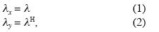
Fractal signals can be either self–similar or self–affine. A self similar signal y = s(x) preserves its shape under a similarity transformation of the two axes x' = λ^αx, y' = λ^α y; while for self–affine signals the two axes need a different scaling x' = λ^α x, y' = µ^βy in order for the shape of y' = s'(x') to remain the same as y = s(x). Images and patterns are often modeled as self–similar fractals, while signals (such as well logs or seismic traces) are considered self–affine (Turcotte, 1997; Mandelbrot, 1999). For example, if the scaling factor of x is λ_x = 3, while for y it is λ_y = 2, we can write (Turcotte, 2002):

with

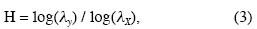
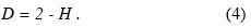
where H is the Hurst exponent. However, the fractal dimension of the trace is related to the Hurst exponent as (Barton and La Pointe, 1995)

 

1.3. Geophysical well logs

Geophysical well logs are of basic importance in identifying hydrocarbon reservoirs. The technique, widely used since 1927, consists of lowering measuring instruments to the borehole and recording the instrument response as function of depth (Johnson and Pile, 2002). The measurements can be classified in three broad categories: electric, nuclear, and acoustic. All of them are, in some particular and indirect way, dependent on the rock–physical properties, as well as on the lithology, porosity, shale content, grain size, water saturation and permeability, among others. All this information is essential to evaluate the productivity of a given formation. An important aspect of this evaluation is the prediction of porosity and permeability based on log data, and to extrapolate these values away from the well (Bassiouni, 1994).

 

1.4. Fractal analysis of well logs

The reconstruction of the HC reservoir geology from core–, well–log–, and 2–D or 3–D seismic data obtained at different scales is the basic challenge facing petroleum industry. An efficient way to integrate such multiscale information, taking into account their temporal and spatial variability, is based on the analytic techniques of fractal geometry. The method is especially useful in describing the spatial heterogeneity of geologic patterns, and has been documented to significantly improve the chances of HC exploration and production (Barton and La Pointe, 1995). When applied in petroleum geology, these novel techniques permit a fractal simulation of the fractured reservoirs, and extraction of the fractal behavior of their structural and sedimentological properties (Barton and La Pointe, 1995, Chap. 12). Fractal geometry provides the adequate framework to analyse typical well–logs, and to model reservoir structures (Tubman and Crane, 1995). Both seismic– and well–log interpretations can be made more precise by assuming that the observed noise, which obeys certain scaling laws, has an inherent fractal nature (Todoeschuck, 1995). This realization suggests to directly analyse "raw" data, wihout the necessity of filtering out noise (Oleschko et al., 2003).

A scale–invariant process can be described by means of its statistical distribution which has a special form, called "power law" (or "fractal–", or "Pareto–", or "hyperbolic distribution"; Korvin, 1992; Mandelbrot, 2002; Turcotte, 2002). Such power–law–type distributions, as well as the scale invariance, are typical in several processes encountered in earth sciences. One of the best example is porosity distribution in sedimentary reservoirs (Turcotte, 2002).

 

1.4.1. Regular fractals

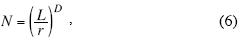
Fractal distributions, because of their intermittent and discontinuous nature, do not completely fill out the Euclidean space (E) but contain a characteristic pattern of gaps or holes (Mandelbrot, 1983). The fractal dimension is a parameter that quantitatively describes these distributions. As it is well known, if we want to cover completely a regular E–dimensional Euclidean object, embedded in a spatial domain of size L, by using smaller objects of size r « L, we shall need a number N of these small objects to do this, where

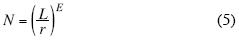
(Hewett, 1986). For example, to cover a L–length linear segment (E = 1) with r = L/3 length–intervals, one needs small "yardsticks". Similarly, we need 9

squares of side L/3 to cover a square (E=2) of side L, and 27 cubes of side L/3 to cover a cube (E=3) of side L. In case of fractal objects however, which do not fill out the space gaplessly, the number of r–size objects required will scale as

where the fractal dimension D is a fractional value, satisfying D < E. A well–known example for a deterministic regular fractal is the Sierpinski carpet. It is constructed by starting out from a large equilateral triangle, dividing it to 4 smaller triangles, and omitting the inverted middle one (Mandelbrot, 1983). Repetition of this step at gradually smaller scales will result in a fractal object of dimension

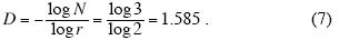
Note that D < 2, that is the object's dimension is less than that of the embedding space. The basic property of this object, which is apparent at first sight, is its scale–invariance. With a proper magnification, a small sub–triangle of any scale can be made identical with the entire object (Mandelbrot, 1983; Korvin, 1992).

 

1.4.2. Statistical fractals

In addition to the "deterministic" fractals, it has been found (Hardy, 1992) that statistical (or "random") fractals are even more useful to model natural phenomena. In case of statistical fractals, the mean value, standard deviation, covariance and spectral density (Isaaks and Srivastava, 1989) of their measurable properties scale with the object size according to a power law.

Two statistical fractal models are especially important for well log analysis: the fractional Brownian motion (fBm) and the fractional Gaussian noise (fGn) (Wornell, 1996). For the fBm the standard deviation of the process grows as a fractional power of the observation time. For the fGn, its covariance function is hyperbolic.

Hewett (1986) first suggested to model well logs using statistical fractals, such as fBm and fGn. He applied the model to study the density log from a sandstone formation. He normalized 2189 data to zero mean and unit variance, and observed that their empirical probability distribution function (pdf) was narrower than a Gaussian pdf, and it was slightly skewed. Then he applied rescaled range analysis (Hurst et al., 1965), which is a basic fractal analysis tool, to the normalized log and obtained a Hurst exponent 0.855 which indicated that the density log was a self–affine fractal with dimension D = 2 – H = 1.145. He also computed the power spectral density of the normalized log. For fGn, the high–frequency part of the power spectrum fell off as a β power of frequency. From the double logarithmic plot of the spectrum Hewett got a slope β = 0.7 which, using β = 2H – 1 (Korvin, 1992) yields again H = 0.855. As a third check of the log's fractality, he also calculated the semivariogram of the sequence that gave 2H= 1.71, in accord with the other estimates.

Having established that the porosity distribution around a borehole has a fractal pattern, the next practical step would be to evaluate how does this affect the fluid transport in the reservoir. For this purpose, Hewett (1986) applied stochastic interpolation of the measured porosity values between boreholes, using the obtained Hurst exponents, and got a realistic contour map of porosity distribution.

In another study (Crane and Tubman, 1990), it was proved that reservoir variability can be modeled by considering the measured logs as stochastic fBm or fGn processes. As well known, the pure Gaussian noise (better known as "white noise"), has the same spectral power for all frequencies. The double logarithmic plot of power versus frequency for such noise is flat, with zero slope:

The previously mentioned two fractal models are related, because the fBm is the integral of fGn. The pure Brownian motion has a spectra decaying according to the hyperbolic law with a log–log slope 2:

 

The spectra of more general fractal noises decay as

It follows from the previous discussion that the larger the value of β, the smoother the corresponding time series graph. Consequently, the fBm is always smoother than the fGn. There are many natural phenomena (from coast–lines, topographies and river levels to voice and music) whose spectra are simply 1/f, lying between the 1/f⁰ and 1/f² processes (Feder, 1988).

The exponent (–β) has a direct connection with the fractal dimension (Mandelbrot, 1983). If the β values are in the range –1 < β< 1, the trace can be considered as fGn (fractional Gaussian noise); if 1 < β <3, it should be modeled as fBm (fractional Brownian motion).

More recently, Hardy (1992) has gone much beyond of Hewett's (1986) ideas of fractal well–log analysis. He studied core samples from boreholes and found a fractal behavior characterized by the same Hurst exponent H as in case of the corresponding porosity logs. With this H value, he used a multivariant fGn process to generate a core model with fractal porosity distribution. He found that using H determined from the power spectra of the core photos, the computed models reproduced the original images with high accuracy. Also, the model could be applied to generate transverse petrophysical profiles across the reservoir, which were statistically equivalent with the models obtained from boreholes. His analyses of the scaling of transverse porosity and permeability profiles have proved without doubt the effectiveness of the fractal technique.

Crane and Tubman's (1990)–simulation study demonstrated that fractal modeling significantly improves the prediction of a reservoir's productivity. They used the R/S technique for three horizontal wells and four vertical wells in a carbonate formation, and found that all recorded logs can be fit by fGn models, with H fluctuating between 0.88–0.89 in vertical wells, and 0.85–0.93 in the horizontal ones.

The main analytical tool utilized in the present work will also be fGn analysis of the well log data (Arizabalo et al., 2004).

 

1.5. Structure and aim of this study

The main objective of this study is to realize a multiscalar fractal characterization and modeling of the spatial variability of the properties of a fractured reservoir (Cantarell), located in the Gulf of Mexico, using recorded well log data.

We will establish criteria to decide whether the assumptions of fractal behavior, scaling or scale–invariance, are valid models to describe the distribution of reservoir properties with respect to depth and geologic time. In further studies, we plan to utilize these models in order to compare the fractal parameters estimated from transverse profiles with those derived directly from boreholes. The data used are logs from a well drilled off–shore by Petróleos Mexicanos (PEMEX), at southeastern Gulf of Mexico (Figure 1).

We will correlate the calculated rugosities (Hurst exponents) and lacunarities with geology, in order to infer the multiscaling behavior of the petrophysical properties of a naturally fractured reservoir at southeastern Gulf of Mexico.

The fractal analysis is realized by means of the "BENOIT" software, which runs under Windows and has been recommended as a reference program for fractal analysis of both self–similar and self–affine sets (Seffens, 1999). We hope the study will contribute to a better understanding and interpretation of the spatial–temporal variabilities of the indicated off–shore reservoir.

 

2. LACUNARITY

 

2.1. Its definition

Mandelbrot (1982) proposed the concept of lacunarity as a quantitative measure of the distribution of holes or gaps in a texture. It describes the way the pieces of a pattern fill out the space and is a complementary parameter to the fractal dimension, which only specifies the amount of space occupied by an object (Tolle et al., 2003). Frequently, patterns with the same fractal dimension have quite different textures, and in such cases their lacunarity measures can be very different. High lacunarity values are associated with the presence of large gaps. Small lacunarity implies a uniform distribution of pores of similar size.

 

2.2. Its computation for patterns

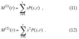
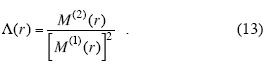
There are several proposed algorithms to compute lacunarity (Gefen et al., 1984; Lin and Yang, 1986). In this work we shall use a simple statistical method for its estimation (Allain and Cloitre, 1991) based on sliding boxes. In this method, a box of side r is placed at the origin of the point–distribution to be analysed. One counts the number of points occupied by the box ("its mass s"), then the box slides one unit step to the right, left, up, or down, until all parts of the pattern has been covered. At each position the "mass" of the box is determined. Next, the procedure is repeated with sliding boxes of gradually increasing size. As a result, one gets the frequency distribution which can be converted to a probability distribution P(s,r) by normalizing with the number of boxes N(r) of size r. Compute the first two moments of the pdf, as (Korvin, 2002):

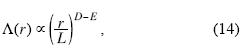
Allain and Cloitre (1991) define lacunarity as

The computed lacunarity is dimensionless and it is related to the width of the histogram of the point distribution (Korvin, 2002).

 

2.3. Scaling of the lacunarity

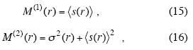
As shown by Allain and Cloitre (1991), the lacunarity Λ(r) scales as a power law

where L is the domain size, r is box size, D is the fractal dimension and E the Euclidean dimension of the embedding space. In a logarithmic (LOG) plot Eq.(14) becomes asymptotically linear, and for self–similar mono–fractals its slope will be D – E (Plotnick et al., 1996). For self–affine sets, recalling the relation D – E = –H between Hurst exponent and fractal dimension, the slope of LOG[Λ(r)] vs LOG(r) will be related to H.

We shall see later, when computing the lacunarity of well logs, which the asymptotic linearity is almost perfect for traces that can be modeled as fractal.

 

2.4. Lacunarity definition for self–affine functions

Another way to represent Eq. (13) is based on the fact that (Korvin, 2002)

 

where <s(r)> is the mean, and σ² the variance of the number of points occupied by a randomly placed r–sized box. Accordingly, Plotnick et al. (1996) defined lacunarity as

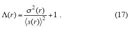
(Note that for a uniform distribution the variance is zero, and the lacunarity is 1.) Equation (17) holds in a range of box sizes from r = 1 up to some maximal size which is a given fraction of the size L of the whole set. Plotnick et al. (1996) suggest r = L /2 as the optimal upper bound. Several conclusions can be drawn from the observed dynamics of the change of lacunarity with box–size:

(1) Scarcely populated point sets have higher lacunarities than dense ones, for the same size of the sliding box.

(2) Larger boxes tend to be more translation–invariant (the second moment decreases with the increase of box size, with respect to the first moment). So, the same set shows lower lacunarity when measured with boxes of increasing size (Plotnick et al., 1996).

(3) For a given box size and given fraction of occupied sites, a larger lacunarity indicates a stronger clustering of the data points (Plotnick et al., 1996).

 

3. FRACTAL AND LACUNARITY ANALYSIS OF A SELECTED WELL

 

3.1. Geology description

Due to reservoir heterogeneity, we selected for fractal analysis the lithologic units of the Cantarell oil field, Gulf of Mexico: Kimmeridgian, Upper Jurassic (JSK), Tithonian, Upper Jurassic (JST), Lower Cretaceous (KI), Middle Cretaceous (KM), and Pal eocene Tertiary Breccia – Upper Cretaceous (BTPKS). [See Angeles–Aquino (1988); Araujo–Mendieta (2004); Basañez (1987) and Pacheco (2002)].

 

3.2. Types of logs used

In the study the following well logs were used:

Neutron porosity (NPHI = Compensated Neutron Porosity (matrix)),

Density (RHOB = Bulk density, DRHO = Delta RHO, PEF=Photoelectric Factor), Resistivity (MSFL = Microspherically Focused Log, Laterolog Deep (LLD) and Shallow (LLS)),

Natural gamma ray (GR = Natural Gamma Ray, CGR = Gamma Ray Contribution from Thorium and Potassium, URAN = Uranium concentration, POTA = Potassium content, THOR = Thorium content) and Caliper (CALI).

 

3.3. Method of analysis

In general terms, the lacunarity calculation followed Mandelbrot (1983). More specifically, we used techniques described in Gefen et al., (1984), Lin and Yang (1986), Allain and Cloitre (1991) and Plotnick et al., (1993, 1996). All lacunarity curves shown were computed by a FORTRAN program based on Eq. (17) (Lozada and Arizabalo, 2003).

 

4.1 Results and discussion of lacunarity of geophysical well logs

We applied lacunarity analysis to Neutron Porosity (NPHI), Density (RHOB, DRHO, PEF), Resistivity (LLD, LLS, MSFL), Natural Gamma Ray (GR, CGR, URAN, POTA, THOR), and Caliper (CAL) logs. All logs belong to a single well in the Cantarell naturally fractured limestone reservoir in the Gulf of Mexico, traversing five geologic strata: Tertiary Paleocene Breccia – Upper Cretaceous (BTPKS), Middle Cretaceous (KM), Lower Cretaceous (KI), Jurassic Tithonian (JST) and Jurassic Kimmeridgian (JSK).

The results are presented as a series of figures, where values of resistivity, fractal dimension and lacunarity are indicated, referred to entire well logs or to specific geologic units studied. Slopes (α) from the LOG(lacunarity) vs LOG(r) plots, and values of the "lacunarity dimension" defined as D(Λ) = will also be given.

Here the term "lacunarity dimension" is used to distinguish between the dimension extracted from the lacunarity and the fractal dimension measured with the BENOIT software (Seffens, 1999).

 

4.1.1. Lacunarity of the neutron–porosity log (NPHI)

Figures 2 and 3 show the neutron porosity log for all the geological layers above mentioned. The entire trace contains 3528 data, with a fractal dimension obtained by the R/S method (Korvin, 1992; Feder, 1988), D_R/S = 1.72, that is to say, a Hurst coefficient H = 2 – D = 0.28, which indicates strong rugosity (Figure 2).

The variation curve of LOG(lacunarity) vs LOG(box size), corresponding to r = 1, gives the maximal lacunarity (Λ(l) = 1.49), this lacunarity is greater than one (topologic limit for an homogenous distribution). The fractal self–similar nature of this log is indicated by the linearity of its behavior through several scales, with high correlation coefficient (R² 0.98) and slope 0.06 (Figure 3).

 

4.1.2. Lacunarity of the density logs (RHOB, DRHO, and PEF)

For density logs, the RHOB lacunarity value for unitary box size, is only Λ(l) = 1.001. As this value is close to the topologic limit, this log shows translation invariance along the entire trace. The fractal dimension obtained by the R/S method for the RHOB trace is 1.716. The function's linearity is observed, with a very low slope of 0.0002 and high correlation coefficient (0.96). Consequently, the density values are very uniform throughout the layers.

The lacunarity behavior of DRHO, with Λ(l)=3.05, is similar to the previous one, with a slightly greater absolute slope of 0.16 corresponding to a lacunarity dimension D(Λ)= =2–0.16=1.84 [D_R/S=1.68] with high correlation coefficient 0.99, that is to say, it exhibits a linear behavior for all box sizes used. This dimension (1.84) is remarkably larger than that measured one from trace rugosity (1.68), which confirms the low resolution of density methods with respect to lacunarity. For PEF, Λ(l)=1.07 the absolute slope is 0.01 (with R²=0.967), which lies between the previous values.

The density tools are interpreted as low sensitivity techniques with respect to lacunarity because of the trace homogeneity.

 

4.1.3. Lacunarity of resistivity logs (MSFL, LLD, and LLS)

MSFL logs (Figures 4 and 5) detected strong resistivity variations in the different layers. The lacunarity value for the entire trace is high, approaching the maximum lacunarity value for r = 1, Λ(l) = 2.92. The absolute slope is 0.13, with R² = 0.8, giving D(Λ) = 1.87. The fractal dimension measured with BENOIT from these data D_R/S is somewhat less, 1.8.

On the other hand, in Figure 6 an irregular behavior in the LLS log is noted. The log has a fractal dimension smaller than for the previous logs (1.69), but a greater initial lacunarity Λ(l) = 5.06, surpassing many times the topological minimum. In addition, slope breaks are observed in the distribution of lacunarity (Figure 7). The slope (0.22) was greater than in the previous case, with a good linear fit (R² = 0.92), corresponding to a lacunarity dimension of 1.78. The LLS average resistivity throughout the entire log is 379 ohm–m, smaller than the MSFL average resistivity.

For LLD (Figures 8 and 9), Λ(l) = 7.3, which is in fact one of the highest values among the analyzed logs. The slope is also high (0.26 with good linearity, R² 0.96), and gives a lacunarity dimension of 1.74 comparable with the value D_R/S =1.68 measured directly from the trace. This means that the LLD has maximum resolution for the measurement of lacunarity and, consequently, to differentiate between petrophysical details and lithology. The fractal dimension of the LLD log, computed with BENOIT, is 1.68, lower than the dimensions extracted from LLS and MSFL. Average LLD resistivity is 1745 ohm–m.

The lacunarity dimensions D_Λ = 2 – average resistivities, and D_R/S dimensions satisfy the following inequalities:

R_ave(LLD) > R_ave(LLS) < R_ave(MSFL),

Λ(LLD) > Λ(LLS) > Λ(MSFL),

D_R/S (LLD) < D_R/S (LLS) < D_R/S (MSFL).

The inequality observed between the resistivity values LLD and LLS indicates a separation between the deep and shallow resistivity curves, which – combined with the low values of density, implies a possible presence of fractures. Resistivity is directly proportional to lacunarity, while lacunarity shows inverse correlation with the fractal dimension.

The slopes of the LOG(lacunarity) vs LOG(r) plot, are greater in all cases than the Hurst exponents calculated directly from the logs. Nevertheless, fractal dimensions calculated from lacunarity satisfy the same inequalities as found by the R/S method, that is to say:

D_Λ(LLD) < D_Λ(LLS) < D_Λ(MSFL).

 

4.1.4. Lacunarity of natural radioactivity logs (GR, CGR, URAN, POTA, THOR)

Natural radioactivity logs display low values of generalized lacunarity. Lacunarity extracted from gamma ray log (GR) has an initial value near Λ(GR) = 1.28. Linearity is lost for scales approaching r = 52 m. The correlation coefficient is 0.84

For the CGR log, an irregular behavior is observed, because Λ(CGR) = 1.83 with a correlation coefficient of 0.82. Linearity abruptly breaks when r approaches 56 m.

The URAN log has an initial lacunarity near one Λ(URAN) = 1.17, with slight variations along the well. A good linear fit (0.98) is observed, with increasing box size.

The POTA lacunarity distribution Λ(POTA) = 1.77, is similar to CGR, with steep fall, a plateau and then again a smooth fall. The correlation coefficient is lower (0.85).

The THOR log has an even more variable lacunarity: Λ(THOR) = 2.04, with a slope of 0.1 (R² = 0.83). In general, natural gamma ray logs are not sensitive to lacunarity.

 

4. 1. 5. Lacunarity of the caliper log (CALI)

In the LOG(lacunarity) vs LOG(r) plot for CALI, the slope is very low (0.006). This indicates a great homogeneity of values. We found linear behavior at almost all scales, up to box sizes near to 152 m, Λ(CALI) = 1.03.

 

4.2. Strata lacunarity for the resistivity logs

 

4.2.1. Lacunarity for the LLD log by strata (BTPKS, KM, KI, JST, JSK)

The lacunarity data calculated from the LLD log were correlated with the lithology of the geological layers of interest. For the Tertiary Breccia – Upper Cretaceous (BTPKS), the lacunarity Λ(l) reached its maximum value of 7.43, with fractal dimension D_R/S of 1.62. This layer is considered a hydrocarbon reservoir.

The fitted slope of LOG(r) vs LOG(lacunarity) plot is 0.33, with R² = 0.96. The lacunarity dimension equals 1.67. The lacunarity curve has two slope breaks around 30 m and 150 m the average resistivity for the BTPKS is 302 ohm–m.

For Middle Cretaceous (KM), the generalized lacunarity value is also high (7.01), with fractal dimension 1.67. Figure 9 shows large gaps between the resistivity highs. The slope is 0.31 with R²=0.97. The fractal dimension extracted from the lacunarity curve is 1.69 (D_R/S =1.67). The average resistivity for this geological unit is 320 ohm–m.

The maximum generalized lacunarity of 9.88 (LLD log), corresponds to the Lower Cretaceous (KI), here the fractal dimension D_R/Sequals 1.76. The high–resistivity values are located in specific zones of the geologic unit, with good linear fit (0.94) and slope 0.22, yielding the lacunarity dimension D_Λ = 1.78, very similar to the D_R/S . The average resistivity for the KI is 247 ohm–m.

For the Tithonian (JST), the lacunarity value decreases to 4.3, and the fractal dimension to 1.7. The slope is relatively low (0.13) and the linear fit is not so good (R² = 0.76). The lacunarity dimension is 1.87, significantly greater than D_R/S. The average resistivity is 1669 ohm–m. This layer corresponds to the hydrocarbon source rock.

In the Kimmeridgian (JSK), the LLD log has a similar behavior as in the previous layer. The generalized lacunarity is 3.09 (lowest in the interval) and the fractal dimension is also relatively low (1.56). The lacunarity curve shows a slope break, but has a meaningful linear fit (slope = 0.26, R² = 0.92), giving a lacunarity dimension of 1.75. The resistivity in JSK is high (5109 ohm–m).

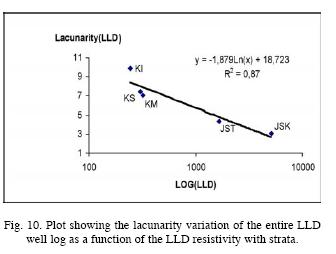
Figure 10 shows an inverse linear behavior of the LLD resistivity in function of lacunarity. It is observed that the corresponding Cretaceous data (KS, KM, KI) tend to cluster in the upper left region of the straight line, corresponding to high lacunarity and medium resistivity. In contrast, the Jurassic data (JST, JSK) occupy the other side of the straight line, with low lacunarity and high resistivity. The Cretaceous data correspond to reservoir rocks, the Jurassic to source rocks: the differences in their lacunarities and fractal dimensions extracted from the resistivity logs are clearly observed (Figure 10).

 

4.2.2. Lacunarity for the LLS resistivity log by strata (BTPKS, KM, KI, JST, JSK)

For the shallow resistivity log (LLS) in BTPKS the lacunarity is lower (Λ( 1) = 1.34) than the previously discussed values, with a relatively homogeneous resistivity distribution. The R/S fractal dimension is also low, D_R/S = 1.61. Resistivity variation is smaller than 100 ohm–m (with an average of 29 ohm–m). The slope of the lacunarity curve is also low (0.06) with R² = 0.97.

In the Middle Cretaceous (KM), the shallow resistivity distribution (LLS) appears homogeneous, with low lacunarity, similar to the previous one (1.34) and a fractal dimension slightly greater than in the preceding case D_R/S = 1.67). The maximum resistivity is smaller than 100 ohm–m, the average being 40 ohm–m. The slope of the lacunarity curve is low (0.08), with R² = 0.93.

For the Lower Cretaceous (KI), the lacunarity decreases further (Λ(l) = 1.15), with a simultaneous increase of fractal dimension (D_R/S= 1.73). The average resistivity is 37 ohm–m. The distribution tends to be homogeneous, the slope is low (0.024), with R² = 0.93.

In the Tithonian (JST), the lacunarity value (1.67) increases towards the medium and lower parts of the interval. The maximal resistivity reaches 1500 ohm–m, with an average of 294 ohm–m. The fractal dimension remains practically the same as in the previous layer (D_R/S= 1.73). Given the nature of the resistivity distribution, with high local values, the lacunarity curve presents slope breaks at box sizes greater than 30 m. There is low slope (0.09), with R² = 0.89.

The LLS log changes radically in the Kimmeridgian (JSK), where its lacunarity increases (Λ(l) = 1.92) and the fractal dimension decreases (D_R/S) = 1.43). The resistivity maximum is close to 5000 ohm–m, but the average resistivity is only 1212 ohm–m. The lacunarity function has slope breaks at box size 80 m, for which the slope increases (0.12), with R² = 0.86.

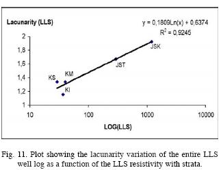
Figure 11 displays the relation between lacunarity and resistivity by geological unit. For Cretaceous data, the points are clustered in the range of low values of lacunarity and resistivity; for the Jurassic in relatively high values of both lacunarity and resistivity.

The LLS log should be considered as of low sensitivity and not apt for the exact calculation of fractal parameters of contrasting geologies. As a consequence, the tendency of the lacunarity change is inverse to that observed in Figures 10 and 11.

 

4.2.3. Lacunarity for the MSFL resistivity log by strata (BTPKS, KM, KI, JST, JSK)

In the Upper Cretaceous (BTPKS) the micro–spherically focused resistivity log (MSFL), is heterogeneous, with high lacunarity (Λ(l) = 6.59) and an R/S fractal dimension equal to 1.64. The resistivity's upper limit is 2000 ohm–m, with an average of 91 ohm–m. The lacunarity function is approximately linear with scale, having a high slope (α 0.24), with R² = 0.96, resulting in a lacunarity dimension 1.76, close to D_R/S.

For the Middle Cretaceous, the lacunarity decreases (to 3.77), but the fractal dimension increases (D_R/S= 1.86), indicating increased rugosity, measured by the Hurst exponent (H = 2 – D = 0.15). The upper limit of the resistivity values is again 2000 ohm–m with an average of 178 ohm–m. The slope ( 0.18) in this particular case approaches the value of H, resulting in a D_Λ = 1.82. The linear fitting is excellent (R² = 0.94).

The generalized lacunarity in the Lower Cretaceous is Λ(l) = 3.18, with fractal dimension D_R/S = 1.65. The resistivity remains under 500 ohm–m, except a few peaks of approximately 1500 ohm–m. The average is 92 ohm–m. Such a distribution produces a curve that smoothly descends, indicating some tendency for homogenization for large box sizes. Consequently, the fit is poor (R² = 0.77), and the low slope (0.09) causes a significant difference between the lacunarity dimension and D_R/S.

The distribution of resistivities is more homogeneous in the Tithonian, where lacunarity significantly decreaseses (Λ(l) = 1.88) and fractal dimension increases (D_R/S) = 1.9). The resistivity remains below 2000 ohm–m, with an average of 677 ohm–m. The lacunarity curve has slope breaks, indicating multifractal behavior. The correlation coefficient is low (R² = 0.77) and the slope is also low (0.07). Nevertheless, the MSFL method is still more sensitive to lacunarity variations than the LLS.

In the Kimmeridgian, the lacunarity decreases still more Λ(l) = 1.59, with D_R/S= 1.85. The upper resistivity limit is 2000 ohm–m, the average is 880 ohm–m. There are slope variations at box sizes 150 m, the linear fit produces a low slope (0.08), with R² = 0.86.

As is the case of Λ extracted from the LLD logs, the lacunarity values in the KS, KM and KI strata are clustered in the region of high lacunarity and low resistivity, contrary to those of JST and JSK, where they have low lacunarity and high resistivity.

 

4.3 Lacunarity of different log types as function of the radial penetration depth

Plotting the absolute value of the slope versus generalized lacunarity Λ(l) for each geophysical log, we obtain Figure 12, where it is evident that with greater lacunarity, better resolution of each method is observed. The slope obtained with this linear fit (0.3), shows the behavior of lacunarity scaling.

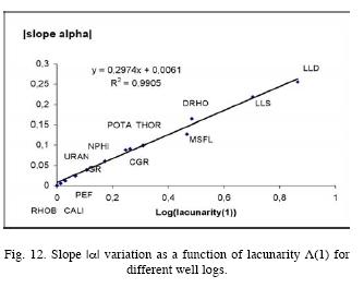
In the plot, the density log (RHOB) has the lowest resolution, the LLD resistivity log has the greatest resolution. The lacunarity varies as function of the resolution of each logging method. Lacunarity increases in the following order for the various logs: RHOB, CALI, PEF, URAN, GR, NPHI, POTA, CGR, THOR, MSFL, DRHO, LLS and LLD. This can be explained by considering the radial penetration of each method. We can imagine that around the well, five cylindrical layers with different radius L exist, at increasing distances from the wall of the borehole.

The RHOB, CALI, PEF, URAN, GR, POTA and THOR logs collect information in nearby cylinders of about 15 cm radius. The MSFL log has greater radial penetration, of approximately 50 cm (corresponding to the flushed–out zone). In case of the DRHO log, the corrected density is based on backscattered neutron– and gamma– rays, so the penetration is somewhat greater than of the previously mentioned RHOB log, because of the higher energy of neutrons. The LLS log is focused on the intermediate zone, that is to say, between 50 cm to 1 m, so that L 75 cm. Finally, the information of the LLD comes from a maximum radius that reaches 1 m or more. By Eq. (14), the variation of lacunarity obeys a scaling law:

where r is the box size, L is the system size. As D < E, and the system size of the well logs increases in the exact order previously mentioned (for RHOB, this is a region of 15 cm diameter around the borehole and for LLD greater than a meter), the scaling law (14) explains the observed systematic increase of lacunarity.

 

5. CONCLUSIONS

We presented results of fractal and lacunarity well logs analysis. In a well traversing a carbonate reservoir of the Gulf of Mexico, different logs were subjected to fractal and lacunarity analyses (NPHI, RHOB, DRHO, PEF, LLD, LLS, MSFL, GR, CGR, URAN, POTA, THOR and CALI). Through the mathematical definition of lacunarity, it has been found that the resistivity logs (LLD, LLS, and MSFL) have larger lacunarity than other logs. Lacunarities and fractal dimension extracted from the resistivity logs are clearly observed. Cretaceous data (KS, KM, and KI) correspond to high lacunarity and medium resistivity. In contrast, Jurassic data (JST, JSK) are associated with low lacunarity and high resistivity. The Cretaceous data correspond to reservoir rocks, the Jurassic to source rocks. For all analyzed logs, it has been shown that geology (BTPKS, KM, KI, JST, JSK) decisively affect the fractal dimension and lacunarity of the formations' stratigraphic properties. Some investigation is in progress in order to develop a general theory that explains the lacunarity variation as function of the resolution of each logging method.

 

ACKNOWLEDGMENTS

This work was partly supported by the Instituto Mexicano del Petróleo. The contribution of PEMEX Exploración – Producción is gratefully acknowledged. Authors appreciate the useful suggestions made by the anonymous referees that improved the manuscript quality.

 

BIBLIOGRAPHY

ALLAIN, C., and M. CLOITRE, 1991. Characterizing the lacunarity of random and deterministic fractal sets. Phys. Rev. A, 44, 6, 3552–3558.        [ Links ]

ÁNGELES–AQUINO, F., 1988. Estudio estratigráfico–sedimentológico del Jurásico Superior en la Sonda de Campeche, México. Rev. Ing. Petrol. Vol. XXVIII (1). 45–55.        [ Links ]

ARAUJO MENDIETA, J., 2004. Evolución Tectono–sedimentaria reciente y su relación con las secuencias estratigráficas del Neógeno en el Suroeste del Golfo de México. Tesis doctoral. Posgrado en Ciencias de la Tierra, UNAM. 211 p.        [ Links ]

ARIZABALO, R. D., K. OLESCHKO, G. KORVIN, G. RONQUILLO and E. CEDILLO–PARDO, 2004. Fractal and cumulative trace analysis of wire–line logs from a well in a naturally fractured limestone reservoir in the Gulf of Mexico. Geofís. Int., 43, 3, 467– 476.        [ Links ]

BARTON, C. and P. R. LA POINTE, 1995. Fractals in Petroleum Geology and Earth Processes. Plenum Press, New York.        [ Links ]

BASAÑEZ, L. M. A., 1987. Estudio estratigráfico sedimentológico de las rocas del Cretácico y Terciario Inferior en pozos del área Marina de Campeche. Instituto Mexicano del Petróleo, México. Informe (Unpublished).        [ Links ]

BASSIOUNI, Z., 1994. Theory, Measurement, and Interpretation of Well Logs. SPE Textbook Series, 4. 372 p.        [ Links ]

CRANE, S. E. and K. M. TUBMAN, 1990. Reservoir variability and modeling with fractals. SPE Paper 20606, SPE Ann. Tech. Conf., New Orleans.        [ Links ]

FEDER, J., 1988. Fractals. Plenum Press, New York and London.        [ Links ]

GEFEN, Y., Y. MEIR, B. B. MANDELBROT and A. AHARONY, 1983. Geometric implementation of hypercubic lattices with noninteger dimensionality, using low lacunarity fractal lattices. Phys. Rev. Lett. 50, 145–148.        [ Links ]

GEFEN, Y., A. AHARONY and B. B. MANDELBROT, 1984. Phase transitions on fractals, III. Infinitely ramified lattices. J. Phys. A: Mathematical and General Phys. 17, 1277–1289.        [ Links ]

HARDY, H. H., 1992. The generation of reservoir property distributions in cross section for reservoir simulation based on core and outcrop photos. SPE Paper 23968, presented in SPE Permian Basin Oil and Gas Recovery Conf., Midland, Texas.        [ Links ]

HARDY, H. H. and R. A. BEIER, 1994. Fractals in Reservoir Engineering. World Scientific, Singapore. 359 pp.        [ Links ]

HEARST, J. R., P. H. NELSON and F. L. PAILLET, 2000. Well Logging for Physical Properties, 2^nd edition: Wiley and Sons, Inc., New York, 492 pp.        [ Links ]

HEWETT, T. A., 1986. Fractal Distributions of Reservoir Heterogeneity and Their Influence on Fluid Transport. Society of Petroleum Engineers (SPE) Paper 15386, presented in SPE Ann. Tech. Conf., New Orleans.        [ Links ]

HURST, H. E., R. P. BLACK and Y. M. SIMAIKA, 1965. Long–Term Storage: An Experimental Study. Constable, London.        [ Links ]

ISAAKS, E. H. and R. M. SRIVASTAVA, 1989. An Introduction to Applied Geostatistics. Oxford University Press, New York.        [ Links ]

JOHNSON, D. E. and K. E. PILE, 2002. Well Logging in Nontechnical Language, 2^nd edition. PennWell.        [ Links ]

KORVIN, G., 1992. Fractal Models in the Earth Sciences. Elsevier, Amsterdam.        [ Links ]

KORVIN, G., 2002. Tutorial on Lacunarity. UNAM. Mexico City. Unpublished Lecture Note.        [ Links ]

LIN, B., and Z. R. YANG, 1986. A suggested lacunarity expression for Sierpinki carpets. J. Phys. A 19, L49–52.        [ Links ]

LOZADA, M. and R. D. ARIZABALO, 2003. Lacuna. for. Unpublished Software. Instituto Mexicano del Petróleo.        [ Links ]

MANDELBROT, B. B., 1982. The Fractal Geometry of Nature. Freeman, San Francisco.        [ Links ]

MANDELBROT, B. B., 1983. The Fractal Geometry of Nature. W.H. Freeman and Co., New York, 468 p.        [ Links ]

MANDELBROT, B. B., 1999. Multifractals and 1/f Noise: Wild Self–Affinity in Physics. Springer–Verlag. New York.        [ Links ]

MANDELBROT, B. B., 2002. Gaussian Self–Affinity and Fractals: Globality, the Earth, 1/f Noise, and R/S. Springer–Verlag. New York.        [ Links ]

OLESCHKO, K., G. KORVIN, B. FIGUEROA, M. A. VUELVAS, A. BALANKIN, L. FLORES and D. CARREON, 2003. Fractal radar scattering from soil. Physical Review E, 67, 041403–1:041403–13        [ Links ]

PACHECO, C., 2002. Deformación transpresiva miocénica y el desarrollo de sistemas de fracturas en la porción nororiental de la sonda de Campeche. Tesis de Maestría en Ciencias (Geología). Posgrado en Ciencias de la Tierra, UNAM. 98 p.        [ Links ]

PLOTNICK, R. E., R. H. GARDNER and R. V. O'NEILL, 1993. Lacunarity indices as measures of landscape texture. Landscape Ecology. 8, 201–211.        [ Links ]

PLOTNICK, R. E., R. H. GARDNER, W. W. HARGROVE, K. PRESTEGAARD and M. PERLMUTTER, 1996. Lacunarity analysis: A general technique for the analysis of spatial patterns. Physical Review E, 53, 5, 5461–5468.        [ Links ]

SCHLUMBERGER, 1984. Evaluación de formaciones en México: México, D.F., Schlumberger Offshore Services–PEMEX. Marmissolle–Daguerre, D., coordinador.        [ Links ]

SEFFENS, W., 1999. Order from chaos. Techsighting software. Science. 285, 5431, 1228.        [ Links ]

TUBMAN, K. M. and S. D. CRANE, 1995. Vertical versus horizontal well log variability and application to fractal reservoir modeling. In: Barton and La Pointe, 1995, Chap. 13.        [ Links ]

TODOESCHUCK, J. P., 1995. Fractals and Exploration Geophysics. In Chap. 14 Barton and La Pointe, 1995.        [ Links ]

TOLLE, C. R., T. R. MCJUNKIN, D. T. ROHRBAUGH and R. A. LAVIOLETTE, 2003. Lacunarity definition for ramified data sets based on optimal cover. Physica D 179: 129–152.        [ Links ]

TURCOTTE, D. L., 1997. Fractals and Chaos in Geology and Geophysics. Second Edition. Cambridge University Press.        [ Links ]

TURCOTTE, D. L., 2002. Fractals in petrology. Lithos 65, 261–271.        [ Links ]

WORNELL, G., 1996. Signal Processing with Fractals: A Wavelet–Based Approach. Prentice Hall. 177 p.        [ Links ]