


 nueva página del texto (beta)
 Inglés (pdf)
 Artículo en XML
 Referencias del artículo
 Enviar artículo por email
 Citado por SciELO
  Similares en
SciELO
Similares en
SciELO 
 Permalink
1 Introduction
A number of complex tasks are systematically performed by honey bees; a good example of such tasks is collection and processing of nectar 1. The effectiveness and simplicity of the whole process is due to the decentralized decision making approach of honey bee colonies 2. Such swarm intelligence features as autonomy, self-organizing, distributed functioning employed by a bee swarm provided inspiration to solve complex traffic, transportation problems 3,4 and deterministic combinatorial problems in dynamic and uncertain environments 5,6,7. Swarm intelligence algorithms based on the behavior of bees can be classified into two categories: the foraging behavior and the marriage behavior. Algorithms in the first category are inspired by searching for food sources and nest sites, while those of the second category are based on the marriage behavior 8. One of the most important algorithms inspired by the foraging behavior of honey bee swarms is the Artificial Bee Colony (ABC). It was proposed by Karaboga and is used for solving various optimization problems 9,10.
The remainder of the paper is organized as follows. Section 2 presents the original ABC algorithm and its selection scheme. Various selection schemes applied to the ABC are described in Section 3. The experimental results are presented and analyzed in Section 4. The paper is concluded in Section 5.
2 Artificial Bee Colony Algorithm
The ABC is a population based optimization algorithm which is iterative in nature. Basically, the ABC consists of cycles of four phases: the initialization phase, the employed bees phase, the onlooker bees phase, and the scout bees phase. The bees going to a food source already visited by them are the employed bees, while the bees looking for a food source are unemployed. The scout bees carry out search for new food sources, and the onlooker bees wait for the information from the employed bees for food sources. The information exchange among bees takes place through the waggle dance. There is one employed bee for every food source. An employed bee becomes scout when the position of a food source does not get improved through the predetermined number of attempts called "limit". In this way, the exploitation process is performed by the employed and onlooker bees, whereas the scouts perform exploration of the search space 10.
There are three control parameters used in the ABC algorithm: the number of employed or onlooker bees to represent the number of food sources (N), the value of limit, the maximum cycle number (MCN). The main steps of the ABC are as follows.
Step 1. Generate the initial population of solutions
Step 2. Generate new solutions for the employed bees using (3) and evaluate the fitness.
Step 3. Apply the greedy selection process for the employed bees.
Step 4. Calculate the probability values for the current solution using (4) so that the onlooker bee can choose one according to its value.
Step 5. Assign the onlooker bees to the solutions according to the probability, generate new solutions using (3) and evaluate the fitness.
Step 6. Apply the greedy selection process for the onlooker bees.
Step 7. If there is a solution abandoned by the bees, stop its exploitation and replace it with a new solution produced by (1).
Step 8. Memorize the best solution found so far.
Step 9. Check the termination criteria. If not satisfied, go to Step 2, otherwise end.
where
 (2)
(2)
where f i is a specific objection function and f it is a fitness value.
where i, k
where fiti is the fitness value of the ith solution and p i is the selection probability of the ith solution.
2.1 Selection Scheme in the Basic ABC
As explained above, food sources are chosen by the onlooker bees using a stochastic selection scheme in accordance with the probability value pi . The process employs three stages 11:
Calculate the fitness value using (2).
Calculate the probability value using (4).
Choose a food source according to the probability value based on the roulette wheel method.
However, the proportional selection scheme employed in the ABC has two shortcomings viz. reduction in population diversity and premature convergence. Thus, the ABC is not able to maintain the balance between exploration (diversification) and exploitation (intensification) of the search space and is considered as an inefficient algorithm.
3 Description of Selection Schemes
The selection scheme plays an important role in the ABC algorithm as it drives the search space in a proper direction. These schemes may be classified in two categories: proportionate selection and ordinal based selection. In the proportionate selection scheme, individuals are selected on the basis of their fitness values relative to the fitness of others, whereas in the ordinal based scheme, individuals are selected based on their rank in the population. The rank is determined in accordance with their fitness values. The schemes presented in this paper except the proportional selection in the basic ABC are covered in the ordinal based selection category. In this work, we performed experiments on the ABC using different selection schemes. The details of the schemes are given in what follows.
3.1 Tournament Selection
This selection scheme works by holding a tournament of N individuals chosen from the population, where N is taken as the tournament size 11,12,13,14. The fitness values of individuals are compared and some score (say, s) is assigned to the best one. The process is repeated till the best in the population achieves the highest score. The individuals are then selected according to the probability using the following equation:
3.2 Truncation Selection
This selection scheme assigns equal selection probabilities to the μ best individuals selected in a population of size λ and is equivalent to (μ,λ)-selection used in evolution strategies 12,15,16. The selection probabilities are given as
 (6)
(6)
3.3 Disruptive Selection
This scheme introduces the concept of normalized-by-mean fitness function. The idea is to give more chances to better and worse solutions in comparison to moderate solutions so that the population diversity can be improved 11,17,18. The selection probability is calculated as follows:
where fiti, is the fitness value of the ith solution and Pi is the selection probability of the ith solution. The fitness function is given by
where f
i is a specific objective function,
3.4 Linear Dynamic Scaling
In order to improve the performance of the proportional selection, it is combined with a scaling technique called linear dynamic scaling 12. The dynamic scaling is introduced to favor better individuals resulting in improved population fitness over generations. The selection probability is given by
where S
f
=
3.5 Linear Ranking
In this scheme, the ranks are assigned to the individuals based on their fitness values. The individual having the worst fitness is assigned rank 1 and the best fitness is assigned rank N. The method uses a linear function to calculate selection probabilities according to the rank of individuals 12,16:
To satisfy the constraints, two conditions must be fulfilled:
η+ = 2- η- and η- ≥ 0.
3.6 Sigma Truncation
In order to improve the fitness of a population, low fitness individuals are discarded using the standard deviation of fitness values before scaling them. This scheme ensures the selection of good fitness individuals 19,20. The fitness values of individuals are calculated as
where
3.7 Exponential Ranking
In this scheme, ranks are assigned to the individuals similar to linear ranking. The difference lies in exponential weighing of ranked individuals to compute probabilities as follows 12,16:
where c<1, an indicative of the selection probability of the best individual.
4 Experimental Results and Discussions
4.1 Test Problems
Six benchmark functions were used for simulation to evaluate the performance of various selection
schemes in the ABC. These functions are the following ones:
i) Sphere function:
ii) Rosenbrock function:
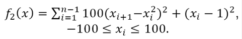 (14)
(14)
ii) Rastrigin function:
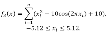 (15)
(15)
iv) Griewank function:
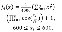 (16)
(16)
v)Ackley function:
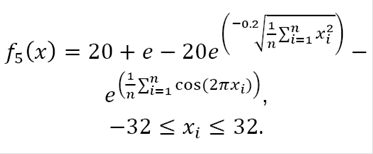 (17)
(17)
vi) Schwefel function:
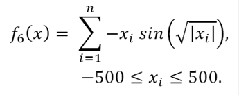 (18)
(18)
4.2 Experimental Settings
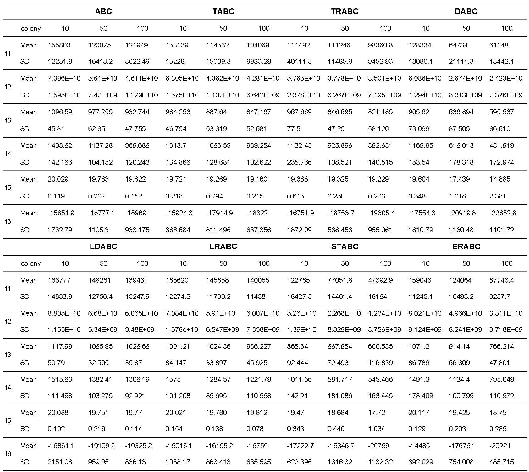
The algorithms for various selection schemes are implemented using MATLAB R2012a on an Intel (R) Core (TM) i3 CPU 3.06 GHZ with 4 GB RAM. In the following tables, ABC represents the original proportional scheme. TABC means the tournament selection, TRABC represents the truncation selection, DABC is the disruptive selection, LDABC is the linear dynamic scaling, LRABC means the linear ranking, STABC represents the sigma truncation, and ERABC is the exponential ranking scheme.
The experiments were performed on the six benchmark functions given above. In all the experiments, the limit was put to 100, and the values present the results of 10 runs (except Table 5 where runs=100). Alongside with comparing the mean values and standard deviations of the function values, the values of selection intensity, success rate, reproduction rate, and loss of diversity were also calculated.
4.3 Effect of Dimensions
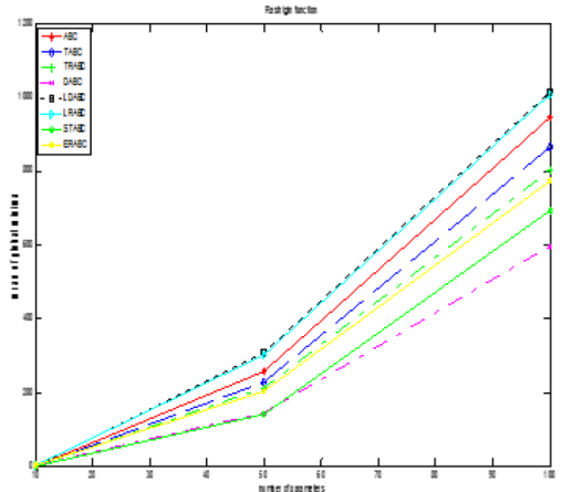
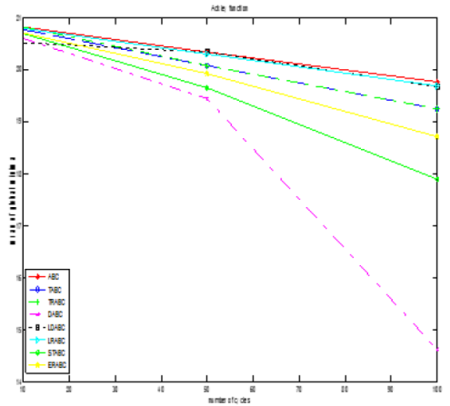
We performed simulations on modified ABC algorithms to analyze the effect of varying dimensions of the problem. The colony size, maximum cycles, and limit were fixed as 100. The performance of all ABC algorithms deteriorated as the dimension of the problem was increased (10, 50, 100).
The results in Table 1 show that STABC generated better results for Rastrigin and Ackley functions followed by LDABC for Sphere and Griewank functions in less dimensions, i.e., 10. Again, STABC produced excellent results with an increase in dimensions up to 50. However, DABC had superior performance for 100 dimensions. From Fig. 1 (a), we can see that the increase in dimensions makes the convergence of DABC method better for Sphere function and also for Rastrigin function as given in Fig. 1 (b).
Table 1 Results of algorithms (varying parameters) [Colony size=100, Limit=100, Max Cycles=100, Runs=10]


4.4 Effect of Cycles
We analyzed the performance of the ABC algorithms by varying the maximum number of cycles. The experiment was repeated for the six benchmark functions as given in Table 2.
The obtained values prove better results for the sigma truncation scheme on Sphere, Rosenbrock, Rastrigin, and Griewank functions. Figs. 2(a) and 2(b) prove better results of STABC on Rosenbrock function and of DABC on Ackley function. For a less number of cycles, i.e. 10, LDABC shows the best performance.
Table 2 Results of algorithms (varying maximum cycles) [Colony Size=100, Limit=100, Parameters=100, Runs=10]


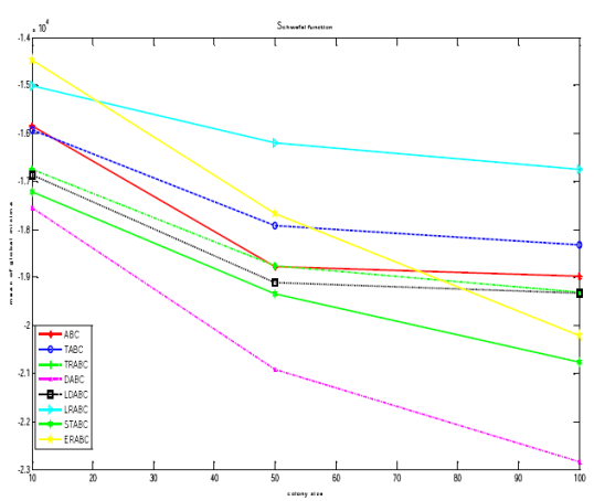
4.5 Effect of Colony Size
In the next experiment, we determined what size of population is suitable to generate better results. The experiment was conducted for all six test problems. Table 3 presents better results in case of STABC on Rosenbrock, Griewank functions, and in case of DABC on Rastrigin, Ackley, Schwefel functions for varying colony sizes.
Table 3 Results of algorithms (varying colony size) [Limit=100, Parameters=100, Max Cycles=100, Runs=10]
For a small colony size of 10, the results of TRABC are good on Sphere function. The performance of DABC got improved with an increase in the colony size as given in Figs. 3(a) and 3(b).

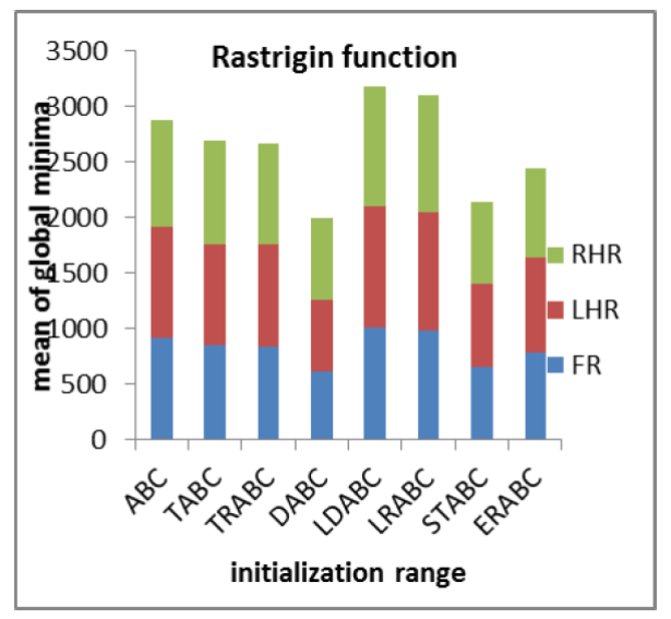
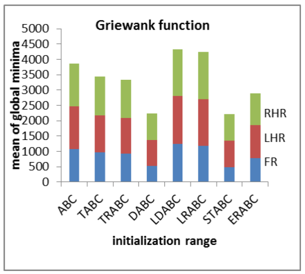
4.6 Effect of Region Scaling
We also investigated the effect of initializing the solutions in various sub-regions of the search space. There was a possibility of variation in the performance of the algorithms during initialization in the left half and the right half of the search space. The results of the experiments using different selection schemes are reported in Table 4. The aim is to determine the sensitivity of the algorithms in finding global optima under varying initialization ranges. All the ABC algorithms were found to be less sensitive to initial solutions in finding global optima as shown in Figs. 4(a) and 4(b).
Table 4 Results of algorithms (varying initialization range) (FR: Full Range, LHR: Left Half Range, RHR: Right Half Range) [Colony size=100, Limit=100, Parameters=100, Max Cycles=100, Runs=10]

4.7 Statistical Analysis
The proportional selection scheme used in the basic ABC lacks the driving force to attract better individuals which may result in premature convergence and a lack of population diversity. The tournament selection scheme randomly selects a number of N individuals and comparison is made based on their fitness values. The truncation selection scheme assigns equal selection probabilities to some selected best individuals in the population. The linear dynamic scaling scheme works by promoting better than average individuals at the cost of worse than average individuals. The linear ranking scheme is biased to favor the good fitness individuals in the population as the rank is assigned based on the fitness value. The exponential ranking scheme works in a similar manner to the linear ranking scheme except the use of the exponential function in computing selection probabilities.
From Figs. 1, 2, and 3, we can state that the DABC and STABC algorithms prove their effective performance in comparison to other algorithms. The disruptive selection scheme favors both high fitness and low fitness solutions and tends to maintain population diversity. Hence, this scheme improves the worse fitness solutions in concurrence with the high fitness solutions. In the case of STABC, the individuals having the fitness value less than c standard deviations of the average value are discarded, while a large portion of the population having the fitness values within c standard deviations of the average value are favored for selection.
Table 5 presents the analysis of the numerical results obtained with a slight change (i.e. 100 runs) in the experimental setting of subsection 4.2 using various selection schemes. Selection Intensity (SI) also called Selection Pressure measures the degree that drives the algorithm to improve the population fitness. It computes the difference between the population average fitness after and before selection. A high value of SI indicates high convergence rate, i.e. the algorithm is able to find optimal solutions early. Positive values of SI in Table 5 prove improvement in average fitness of the original ABC and the modified ABC algorithms due to selection for all test functions.
Table 5 Results of algorithms (SI: Selection Intensity, SR: Success Rate, RR: Reproduction Rate, Pd: Loss of Diversity) [Colony size=100, Limit=100, Parameters=10, Max Cycles=100, Runs=100].

Success Rate (SR) shows that algorithm is able to obtain a desired function value (i.e. <2) using the given experimental settings. From the table, we can see that the success rate of the TRABC and STABC algorithms gets improved for Rastrigin function, whereas it is comparable to the original ABC for the remaining test functions.
Reproduction Rate (RR) is calculated to represent the ratio of the number of individuals with a certain fitness value after and before selection. A value of RR > 1 means better individuals are favored and bad individuals are discarded by a suitable selection scheme. Table 5 clearly shows that all selection schemes are able to replace bad individuals by better individuals.
Loss of Diversity (Pd) presents the ratio of the individuals of a population that are not selected during the selection stage. It means that Reproduction Rate and Loss of Diversity are
related to each other. The value of Pd should be as low as possible, as a high value of Pd may increase the risk of premature convergence. The values in the table clearly confirm the results.
5 Conclusions and Future Work
In this paper, we compared the performance of the Artificial Bee Colony algorithm combined with different selection schemes on six numerical optimization functions. The simulations were performed by varying the values of different control parameters used in the ABC algorithm in addition to initialization ranges. On the basis of the results obtained, an analysis is made in terms of selection intensity, success rate, reproduction rate, and loss of diversity.
With an increase in the number of dimensions, it becomes difficult to find optimal solutions in all selection schemes. As the number of cycles increases, the algorithms explore and exploit efficiently the search space to provide proper convergence and population diversity. An increase in the colony size also provides an opportunity to find global optima values. The algorithms are also less sensitive to initialization ranges in obtaining optimal solutions.
Positive values of Selection Intensity in all schemes represent an increase in the population average fitness after selection. Success Rate is an indicative of obtaining a desired function value. All selection schemes favored good individuals by assigning the reproduction rate > 1. Similarly low values of loss of diversity support the avoidance of premature convergence. In general, the ABC algorithms combined with different selection schemes perform better on various parameters. In future work, the performance of the ABC can be improved by hybridizing it with a suitable selection scheme and an effective neighbor search technique.

